Hyperdimensional Computing (2): Building an encoder
How to design, build and evaluate an encoder for hyperdimensional computing.
In the previous post, we went over the algebra of hyperdimensional computing (HDC), a computing paradigm where data is processed using very high-dimensional vectors (10K dimensions). In this post, we’ll build an HDC encoder for the tea dataset by looking deeper into how a hypervector is created from its raw JSON fields. I’ll use the example of my favourite tea, Ali Shan oolong (from Taiwan), to illustrate the process.
We used binding to associate values with their roles, followed by bundling to create superpositions of those bound hypervectors. This let us use cosine similarity to compare the resulting hypervectors to find entities associatively.
An encoder is like an adapter that maps the raw data into a hypervector. Designing a good encoder requires domain knowledge, as this informs how the various components of the raw data should be assembled to provide a meaningful representation in high-dimensional space.
For our tea dataset ⤴, the encoder must be built to handle questions like the following:
- Can two tea aroma fields remain similar even when their words don’t exactly match?
- Is an elevation of 1,400 m considered “closer” to 1,200 m than to 500 m?
- How strongly should either of those properties influence the result compared with the class, roast or oxidation values?
From HDC algebra to implementation#
HDC is a broad field that defines the concepts and the algebra we need to work with hypervectors. But in practice, we need a concrete way to represent hypervectors and apply HDC algebra in code. For this project, I used TorchHD ⤴, a thin wrapper over PyTorch that provides tensor types and operations for binding, bundling, permutation and similarity calculation. You don’t have to use TorchHD, though, and there are several alternatives if you want to explore HDC further.1
HDC covers a broader family of algebraic models, often called Vector Symbolic Architectures (VSAs). TorchHD implements several of them, making it a convenient interface for this project. For the tea encoder, we’ll use the Multiply-Add-Permute (MAP) model. MAP represents hypervectors as dense, -dimensional binary () or bipolar () arrays, and provides the primitives for working with them.
Bipolar hypervectors are invertible#
Using a bipolar representation (where all values are ) is especially beneficial for invertibility of binding operations. MAP binds two hypervectors using element-wise multiplication, so every bipolar hypervector is its own inverse (i.e., binding becomes “self-inverse”). If we bind a role hypervector to a value hypervector , multiplying by again recovers the value:
Self-inverse binding is also useful for querying structured representations: the same operation can create an association and retrieve its value when the role is known, without requiring a separate decoder. We’ll see later how this also helps us inspect the evidence contributed by each field and explain the result.
Bundling strengthens the signal#
For similarity search to work, the final tea hypervector must retain a recognizable trace of every field we put into it. We do this by bundling those bound hypervectors (adding them element-wise). This way, coordinates that agree strengthen parts of the sum, while disagreement cancels out elsewhere. Summing the components retains enough similarity to the original hypervectors while also capturing the differences. The visual below shows this across three field components.
During storage (in this case, using LanceDB), we could normalize the sums back to a bipolar hypervector, but doing so mashes all values into +1 or -1, wiping out the relative strengths where the components agree or disagree. To preserve the signal strength, the bundled hypervector is typically stored unnormalized (with the raw sums).
During retrieval, however, cosine similarity performs a form of normalization: it divides the dot product by both L2 norms to calculate a similarity score. This keeps overall vector length from dominating the ranking while preserving each field’s relative influence and allowing us to decompose the bundle later.
A natural question is how many fields a bundle can hold before the signal from any one of them becomes too faint to recover. With only a handful of tea fields, we’re far from that limit, but I ran some experiments to find where it lies in Testing the limits of bundling capacity ⤴, using a 50-item questionnaire.
What goes into a “tea hypervector”?#
The first stage in encoder design involves us explicitly deciding which fields matter to the downstream retrieval task. We’ll encode six fields: aroma, taste, class, oxidation, roast and elevation_meters.
This is the example Ali Shan record, along with its relevant fields:
{
  "title": "Ali Shan",
  "class": "oolong",
  "oxidation": "medium",
  "roast": "none",
  "aroma": [
    "LEMONGRASS",
    "WHITE PEACH",
    "LAVENDER",
    "intoxicating floral aromas reminiscent of lavender and hyacinth",
    "orchard fruits",
    "citrus peel",
    "lemongrass notes"
  ],
  "taste": ["full and buttery texture"],
  "elevation_meters": 1400,
  "elevation_confidence": 1.0
}
Every key-value pair must eventually become a role-value bound pair that we’ll then bundle into a 10,000-dimensional hypervector representing “Ali Shan tea” in high-dimensional space. However, each role-value pair carries a different data type whose qualities we need to preserve in the encoded representation:
| Fields | Relationship to preserve | TorchHD class |
|---|---|---|
class | Categorical (unordered) labels | Random |
oxidation | roast | elevation_meters | Ordinal values or ordered variables | Level |
aroma | taste | Related phrases should remain related | Projection |
TorchHD provides a torchhd.embeddings module, in which Random generates a hypervector with random values (useful for distinguishing unrelated or unordered classes). Level, on the other hand, preserves proximity along an ordered scale, and Projection maps a continuous input (like dense vectors) into hypervector space. Oxidation and roast are discrete levels where order matters, while elevation is a continuous measurement that we discretize into 50-metre bins.
Unordered categories#
This dataset has 5 nominal categories of tea: green, white, yellow, oolong and black. These are distinct labels, where the order in which they appear doesn’t matter to the meaning in the representation. We don’t want to encode them as numbers, because that would imply a relationship between them that doesn’t exist.
We instead assign each class a random bipolar hypervector. In 10,000 dimensions, independently generated hypervectors are almost guaranteed to be near-orthogonal, which means their cosine similarity is close to zero. The encoder uses a global seed of 13, and with this seed, the hypervectors for oolong and black have a cosine similarity of 0.0082, meaning they’re extremely dissimilar in hypervector space.
To make generation reproducible, the global seed, roles and values are hashed together using SHA-256. We then use the result to seed PyTorch’s random number generator. This way, the same input, such as 13|item:class|oolong will always produce the same random-looking hypervector every time, making this a deterministic process.
In this manner, the role class is bound to the value oolong:
It looks just as simple in code:
# hv is the TorchHD hypervector factory instance
value = self.hv.item("class", record["class"])
class_component = bind(self.hv.role("class"), value)
Binding the role to its value preserves the distinction between “this tea belongs to the class oolong” and the same “oolong” token appearing somewhere else.
Ordered categories or ordinal values#
The oxidation, roast and elevation fields need a different treatment because the order of these values carries useful information that our encoding needs to preserve. A low oxidation should be recognizable as being below medium, just as the elevation 1,400 m should be considered lower than 1,600 m, but higher than 500 m. Generating random item hypervectors would throw those relationships away.
TorchHD provides the Level abstraction to handle fields like these, by interpolating between two random endpoints within the 10,000 components. Moving one step along the ordered scale changes only some coordinates of the hypervector, so adjacent levels remain highly similar and gradually diverge as the distance grows. In our tea encoder, we obtain the following similarity results for oxidation and elevation:
| Comparison | Cosine similarity |
|---|---|
low vs. medium oxidation | 0.4898 |
low vs. high oxidation | -0.0094 |
1,400 m vs. 1,450 m | 0.9824 |
1,400 m vs. 500 m | 0.6924 |
The numbers above tell us that low and medium oxidation are moderately close in hypervector space, while low and high are farther apart. Similarly, the elevation levels of 1,400 m and 1,450 m are very close, while 1,400 m and 500 m are still somewhat close, but less so.
For the elevation at which a tea is grown, our dataset uses 61 levels spanning 0 to 3,000 metres in 50-metre steps. Ali Shan’s elevation of 1,400 m maps to the value , which is then bound to the elevation role:
# 1. Build the ordered elevation scale
elevation_levels = Level(
    count=61,
    dimensions=10_000,
    range=(0, 3_000),
)

# 2. Select Ali Shan's level by binning into 50-metre increments
level_index = 1_400 // 50  # 28
elevation_value = elevation_levels[level_index]

# 3. Bind that value to the elevation role
H_elevation = bind(R_elevation, elevation_value)
The range of 0–3,000 m and the 50-metre bin resolution are modelling choices made by us, and is totally subjective. In a different application, we might use finer bins or a continuous encoding.
This bin structure encoded as levels is powerful, because it lets us ask counterfactual questions like this: “Which tea resembles Ali Shan but grows at 1,600 m?” (Recall that Ali Shan grows at 1,400 m). Because each tea’s final hypervector is a sum of bound role-value hypervectors, we can build this kind of query via the same encoder. Here, means the complete elevation contribution, including its weight in the final bundle:
We subtract the old elevation component and add the new one, while the stored Ali Shan hypervector and all its other fields remain untouched.
With one subtraction and one addition, we got a tea “similar to Ali Shan, but grown 200 m higher.” Mi Lan Xiang Lao Cong is a similarly fruity and floral oolong tea from the Guangdong region of China, with notes of lychee, peach, pink grapefruit and a supple, sweet finish. We obtained this result using vector arithmetic directly on the encoded representation and with no encoder changes.
This is why HDC is so powerful: the structured fields become something we can compute with.
Semantic text embeddings#
The aroma and taste text fields contain vocabulary terms that describe the sensory characteristics of the tea, such as orchard fruits, floral and buttery. The encoder itself has no notion of a vocabulary. How can we preserve the meaning of these descriptions in a hypervector representation, so that buttery is recognized as being more similar to creamy than to grassy?
Classical HDC systems often use a codebook, a fixed vocabulary that maps every known symbol to a hypervector. That works well for exact symbols, but a random codebook would treat buttery and creamy as unrelated unless we designed their connection ourselves. With an open-ended vocabulary, we can’t enumerate every possible phrase in advance. We need a way to encode the meaning of phrases that the encoder has never seen before.
The good news is that we already have a solution that’s worked well in RAG: traditional text embeddings that encode semantics via a pretrained embedding model. We can use a model like nomic-embed-text ⤴ to map each aroma and taste phrase to a 768-dimensional text embedding, which gives us a notion of semantic similarity in that space.
Before embedding the text of the taste and aroma fields, we clean up whitespace, remove duplicates and sort the phrases. We embed each phrase separately, then apply mean pooling to the phrase embeddings by taking their element-wise mean:
Here, is the Nomic text embedding for one phrase. Sorting makes the result reproducible, while mean-pooling combines the phrases into one single embedding without making longer descriptions dominate more.
# Standardize Unicode, whitespace and casing first to get `cleaned_phrases`.
# Drop empty strings and sort the phrases into a reproducible order.
phrases = tuple(sorted(phrase for phrase in cleaned_phrases if phrase))

# Embed each phrase separately, producing an (n, 768) array.
stacked = np.stack([self.phrase_embedding(phrase) for phrase in phrases])

# Mean-pool across the phrases to produce one 768-dimensional field embedding.
field_embedding = stacked.mean(axis=0)
We can now find teas similar to Ali Shan tea’s buttery texture via a query such as creamy, even though the words don’t exactly match.
However, we now have a new problem: the text embedding lives in lower-dimensional space, completely distinct from our MAP hypervectors’ 10,000 dimensions.
Project upward to higher-dimensional space#
To bring the text embeddings into the same hypervector space as the other role-value bound hypervectors, we need to do a projection of the 768-dimensional embedding upward to 10,000 dimensions.
One of the ways to do this is to define a fixed Rademacher matrix . A Rademacher distribution is a discrete probability distribution that returns -1 or +1 with equal probability. Each column in the random matrix contains positive and negative signs, which act like votes across all 768 values in the text embedding.
We generate this matrix once when the encoder is initialized, then reuse it for every tea record. To fill the matrix, we make 7.68 million () independent fair-coin flips, placing -1 or +1 in each cell, with a fixed seed to make those draws reproducible. Across 10,000 columns, those “votes” distribute the phrase’s semantics throughout the resulting hypervector.3
Every aroma and taste embedding is multiplied by this shared matrix. Multiplying a Nomic text embedding by a Rademacher matrix returns a array, exactly the dimension we need for our hypervector space.
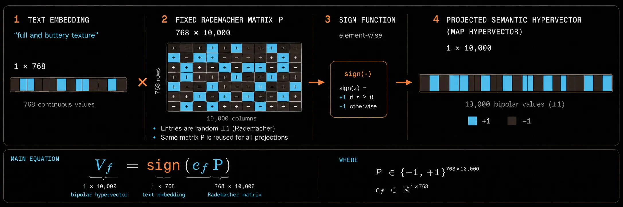
Using the same matrix keeps all the projected results in the same coordinate system, so we can compare them meaningfully.
In code, this is a series of PyTorch operations that multiply the embedding by the Rademacher matrix, then apply a sign function to convert the result to bipolar form:
# Create the fixed 768 x 10,000 Rademacher matrix from the manifest seed.
projection = rademacher_matrix(manifest, hypervector_factory)

# Convert Nomic's embedding to a tensor, then multiply the two matrices.
text_embedding = torch.from_numpy(embedding)
projected = torch.matmul(text_embedding, projection)

# Map every coordinate to +1 or -1, producing a bipolar hypervector.
positive = torch.ones((), dtype=projected.dtype)
value_hypervector = torch.where(projected >= 0, positive, -positive)
Note that the upward projection doesn’t create new semantic information. It simply re-expresses the Nomic text embedding as a higher-dimensional bipolar hypervector that we can then use to compute with, in the same algebraic space as the other fields. The matrix multiplication preserves the embeddings’ neighbourhood structure, while the sign function converts the result to bipolar form.3 The table below shows the cosine similarity between the original Nomic embeddings and the projected hypervectors for a few example phrases:
| Comparison | Nomic embedding | Projected MAP hypervector |
|---|---|---|
buttery vs. creamy | 0.8018 | 0.5952 |
buttery vs. seaweed | 0.6571 | 0.4670 |
The absolute similarity scores change because these are different representation spaces. But the change in meaning remains consistent: creamy remains closer to buttery than it is to seaweed in both. This lets us bind the projected hypervector to its aroma or taste role, so that the final tea hypervector retains a trace of the Nomic model’s representation of sensory characteristics.
Weighting the fields using domain knowledge#
At this point, we have bound, 10,000-dimensional hypervectors that represent each role-value pair from the source data. We can combine them via bundling, but it’s important to remember that they don’t all contribute equally to the notion of a “tea”.
The aroma and taste fields came from human-written descriptions grounded in a human’s sensory experience from the real world, so they each receive a more significant 0.25 fraction of the weight. Elevation is far weaker evidence: it was inferred by an LLM and includes a confidence score (two very different teas can grow at the same elevation), and it’s also a weak proxy for the chemical composition of tea. For fields like this, we reduce the weight.
The final expression to produce the bundle looks like this:
Here, is the confidence in the inferred elevation. There are many other ways we could weight these components. The main takeaway is that HDC lets us bake in whatever domain knowledge we want directly into the encoder’s design, rather than leave those priorities implicit (or rely on the model “learning” those signals from data, like traditional text embeddings).
That’s it, the output of this expression, , is our final tea hypervector! 🍵
Does this work well in practice?#
The encoder is now run over every record in the dataset, producing a 10,000-dimensional hypervector for each tea. To see whether those representations move in sensible directions, it makes sense to run a quick sensitivity analysis.
I made three copies of the Ali Shan oolong tea hypervector, changing only one field in each, and ran each of them through the encoder to generate three “modified Ali Shan hypervectors”. Each one was then searched via cosine similarity against the full dataset of 166 teas. The aim of this study was to see whether the nearest neighbours moved in the expected direction, changing the rankings in a way that made intuitive sense.
-
Raise
elevationto 2,200 m. Changing the elevation of Ali Shan tea from 1,400 m to 2,200 m moved Li Shan, a Taiwanese high-mountain oolong grown at 2,000 m, from rank18to9. Da Yu Ling, another Taiwanese oolong grown even higher at 2,300 m, moved from35to27. Neither became the closest match because elevation carries only part of the final score, but both moved in the expected direction. -
Increase
oxidationto high. Changing oxidation frommediumtohighmoved two highly oxidized Taiwanese oolongs: Bai Hao from rank13to1, and Gabacha Black from rank25to2. Both teas come with darker, fruitier profiles. Because we didn’t change Ali Shan’sclassfromoolong, the results contained more oolongs than black teas. -
Replace
tastewith “crisp and refreshing”. Replacing Ali Shan’sfull and buttery texturewithcrisp and refreshingmoved Sencha Yabukita (a Japanese green tea, very different from Ali Shan oolong tea) from rank93to32. Because the aroma and taste fields are highly weighted in our encoder, the phrase “refreshingly crisp” that appears in the green tea’s description ranks highly, even though the exact phrase in the taste field didn’t match what’s stored in the data.
Overall, these results look quite convincing!
- The encoder responds to changes in individual fields in a way that makes intuitive sense.
- The semantics of the aroma and taste phrases are carried over from the text embedding into hypervector space.
This means that our encoded representation is robust enough to be useful in practice. 🚀
A representation we can reason about#
The encoder is the most important part of an HDC system. Unlike end-to-end representation learning (which learns a representation from data), an encoder is fixed, and its representation is designed upfront, using a combination of domain knowledge and composable operations.
All the structure and tuning knobs in the encoder were baked into the representation itself. This fixed representation enables associative search while giving us explicit control over how it’s designed. We didn’t have to rely on training a model on a dataset of elevation or oxidation, or add hybrid search, reranking and metadata filters around the representation to express those relationships.
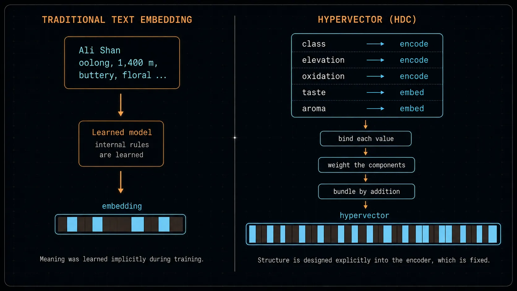
The main limitation of relying on an off-the-shelf text embedding model is that we’re relying on the model’s understanding of the domain and its vocabulary. However, this is the same limitation we also face in any RAG system. HDC doesn’t circumvent that problem, but it does give us a way to combine the text embedding with other structured fields in a way that preserves their relationships and lets us reason about them mathematically.
What’s next: building an online learner#
We now have a fixed encoder for representing teas, but the system is static. It doesn’t yet learn as new data comes along. That’s where a prototype4 comes in: in the HDC literature, a prototype is a hypervector formed by bundling several real-world “training” examples so that it remains similar to what they share.
In the next post, I’ll show how I built a “tea recommender” using a small training dataset of 10–15 teas that I’ve tried and use it to build a “preference prototype”. The teas I liked will help build a positive preference, while the teas I was neutral towards (or disliked) will build a negative one. As new records are added to the training set, the prototype can be updated with the same simple algebra as in the encoder. The sample efficiency of HDC-based learning is quite remarkable, so we can build a useful preference prototype with very few examples.
The learning we’ll be doing is online, i.e., the system can continuously learn as new examples come in. It’s fundamentally different from what we do in deep learning, where the model is retrained offline through a separate training run.
Hopefully, reading this post made you want to build your own encoder. See you in the next post! 🍵
Code#
The best way to understand how the encoder works is to go through the code and build with it yourself. Check out the source repository for the project and give it a star:
Waiting for api.github.com...
Footnotes#
-
TorchHD offers broad HDC/VSA coverage, but it’s a thin PyTorch layer, is lightly maintained, and its package metadata ⤴ still declares
torch>=1.9.0. For a production MAP pipeline, native PyTorch ⤴ is probably the leanest option: binding, bundling, permutation and similarity map directly to multiplication, summation,torch.rolland cosine similarity. VSAX ⤴ provides MAP in the JAX ecosystem when XLA and JIT compilation are attractive. HoloVec ⤴ is a newer multi-backend alternative. hdlib ⤴ is more actively developed, but brings a heavier scientific and Qiskit dependency stack. There’s also HyperdimensionalComputing.jl ⤴ for folks working in Julia, and OxiCUDA ⤴ if you want a modern CUDA alternative in Rust. ↩ -
Zhang et al., “Non-targeted metabolomics study for the analysis of chemical compositions in three types of tea by using gas chromatograph-mass spectrometry and liquid chromatography-mass spectrometry” ⤴, Chinese Journal of Chromatography, 2014, detected 4,420 chemical features in 33 green, oolong and black teas, then confirmed 109 compounds against standards. These included amino acids, carbohydrates, lipids, organic acids, catechins, flavonol glycosides and alkaloids. Unfortunately, the paper doesn’t identify the individual teas behind its 33 samples, so their chemistry can’t be joined directly to this project’s 166 records. ↩
-
Each of the 10,000 columns defines a different yes-or-no test over the entire embedding: after adding its randomly signed contributions, is the total positive or negative? Similar embeddings tend to produce the same answer across many of these tests because small changes usually don’t flip the sign. Their shared pattern across 10,000 coordinates therefore preserves which phrases are close, while no single coordinate carries meaning on its own. The random matrix is generated with a fixed seed, so the same embedding always produces the same hypervector. ↩ ↩2
-
Kleyko et al., “Classification and Recall With Binary Hyperdimensional Computing: Tradeoffs in Choice of Density and Mapping Characteristics” ⤴, IEEE Transactions on Neural Networks and Learning Systems, 2018, defines a class prototype as one hypervector built by bundling its examples. Rahimi et al., “Efficient Biosignal Processing Using Hyperdimensional Computing: Network Templates for Combined Learning and Classification of ExG Signals” ⤴, Proceedings of the IEEE, 2019, shows how these prototypes can be updated incrementally by adding each newly encoded example. ↩