Hyperdimensional Computing (1): The algebra of hypervectors
How hypervectors can produce robust, distributed and composable representations of real-world data.
In his landmark 2009 paper, Pentti Kanerva1 made an insightful observation:
The dimensionality of an entity (a number) and the dimensionality of its representation for computing purposes (a bit vector) are separate issues.
To understand why a representation matters, let’s take the number 27. Mathematically, it’s a scalar (a single point on a number line). However, its representation on a computer requires the binary pattern 11011. It takes two digits to represent it in decimal, but five bits to represent it in binary.
The larger representation is not more meaningful on its own, but it gives a machine built on binary logic gates something more powerful: the ability to operate on the data much more easily. Add an 8-bit representation of 5 (00000101) to an 8-bit representation of 27 (00011011), and we get 00100000, which converts back to the integer 32. The representation is what enables efficient computation over the data.
Hyperdimensional computing (HDC) is a computing paradigm for AI that takes this intuition much further. In HDC, we transform not only numbers, but arbitrary data into hypervectors (10,000 dimensions or more). We can then use a simple algebra to transform, combine and compare them in this high-dimensional space. Importantly, the operations are composable, allowing us to preserve the stored data’s inherent structure. The operations are also reversible, so we can easily recover the raw data from its representation.
Real-world data exists in a high-dimensional space, which can be thought of as a fuzzy manifold. Each data point lies on that manifold, and is represented as a high-dimensional vector (a “hypervector”) that originates at the centroid of the manifold. The algebra in HDC lets us move around the surface in ways that preserve relationships between points. Two points that are close together on the manifold will have hypervectors that are more similar than two points that are far apart.

If this is your first foray into hyperdimensional computing, welcome! In this post, we’ll go over what hypervectors are, what properties they have, and what operations we can perform on them.
High dimensionality: from curse to blessing#
Traditional machine learning tends to view high dimensionality as a curse, where it’s common to resort to dimensionality reduction techniques when working with the data. In contrast, HDC views high dimensionality as a “blessing” rather than a curse. The field of HDC has its roots in cognitive science, where it’s thought that the highly interconnected nature of the brain’s neurons allows for distributed representations of information that exist in a very high-dimensional space, enabling intelligence.
This leads us to one of the most important insights from Kanerva’s paper1: high dimensionality is useful because it gives us a large, distributed representational space that remains closed under a small algebra. And because the algebra exposes composable operations, this lets us easily combine hypervectors to create new ones in various ways, no matter the shape of the original data.
A real-world dataset of tea#
In my previous post about my newfound fascination with loose-leaf tea, I showed how I curated a tea dataset ⤴ that captures various attributes of each tea. It turns out, that dataset is a great way to demonstrate how HDC works. Below is an example JSON record of one of my favourite black teas (Yunnan Dian Hong), from China’s Yunnan province. We’ll walk through a conceptual view of how to work with it using HDC algebra.
{
  "id": 1314971975789,
  "title": "Yunnan Dian Hong",
  "description": "A superb Yunnan black tea made from large leaves and large golden needles offering a smooth, velvety and tasty liquor with comforting aromatic accents: notes of candied fruits, caramel, blond tobacco, malt, moist earth. 1 tsp/250ml 3-4 minutes 90-95°C",
  "aroma": [
    "candied fruits",
    "caramel",
    "blond tobacco",
    "malt",
    "moist earth"
  ],
  "taste": [
    "smooth, velvety"
  ],
  "oxidation": "high",
  "roast": "none",
  "elevation_meters": 1950
}| Fields | Data type | What they capture |
|---|---|---|
description | string | The complete description of the tea |
aroma | taste | lists of strings | Sensory phrases extracted from the description |
oxidation | roast | ordinal categories | Ordered levels describing how the tea was processed |
elevation_meters | number | The elevation at which the tea was grown |
As described in the earlier post, the elevation at which tea grows directly influences its flavour profile. When tea is grown at higher elevations, the cooler conditions slow the plant’s growth, which changes the balance of amino acids and polyphenols in the leaf. This affects the tea’s aroma, taste and mouthfeel, making the elevation number a proxy for a complex set of chemical and sensory properties that aren’t captured in the text description.
Together, numbers, categorical variables and text can describe aspects of the tea more faithfully than text alone. The image below shows, conceptually, how five different kinds of tea (green, white, yellow, oolong and black) might occupy such a hypothetical, shared high-dimensional space. Each example tea is represented by a hypervector pointing toward its data point within the corresponding category.
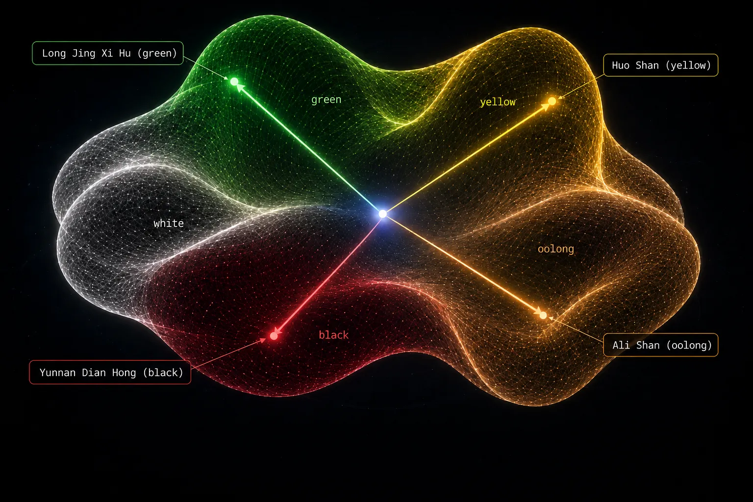
If you’ve ever used vector search or RAG before, this may look familiar. However, the crucial difference is the way the hypervectors are constructed. In RAG, the embeddings are generated by a pretrained model that has learned (from a large amount of data) to encode text into a dense vector space that dissolves any structure in the original data. In HDC, we construct hypervectors using a fixed encoder built with human intuition, and we use a simple algebra that preserves the structure of the data.
Characteristics of hypervectors#
A hypervector is a very long array of numbers (typically 10,000 dimensions) used in HDC to represent and process information. It’s generated by an encoder that maps raw data into a shared, fixed-width hypervector space. Hypervectors have several useful properties that make them suitable for representing complex data in a robust and composable way.
Here, is the value at position , and is the length of the hypervector (typically 10,000 dimensions or more).
For the tea dataset, every property value is mapped into this same fixed-width space. The encoder design is what maps the roles and qualities of the data into the hypervector. We’ll unpack the details of encoder design in the next post of this series. For now, let’s focus on the key qualities of hypervectors themselves.
Independence#
The useful properties of hypervectors only emerge when you have thousands (typically tens of thousands) of dimensions. A 10,000-dimensional space contains possible hypervectors, a stupendously large number. Any data we could represent would fill only an infinitesimally small fraction of that space. Two randomly chosen hypervectors in this space point are almost guaranteed to be near-orthogonal, meaning that their cosine similarity is close to zero.
This gives unrelated concepts plenty of separation. Shared structure can move two tea hypervectors closer together, while arbitrary representations begin with almost no similarity.
Robustness#
Because of its length, a hypervector is robust to noise or corruption. The representation is sufficiently redundant, so changing many values moves it only gradually away from the original. No single value among its 10,000 positions encodes meaning on its own (see the next quality on holistic representation), so flipping a few values doesn’t change its overall meaning.
This distinguishes hypervectors from ordinary binary encodings, where flipping one bit can completely change the represented value.
Holographic behaviour#
A hypervector is holographic and maintains a holistic representation because its information is distributed throughout the entire pattern. Kanerva describes this as the most efficient use of redundancy: information is spread “equally” over all 10,000 components, so the representation degrades in proportion to how many values fail, regardless of where they sit. This is very different from binary numbers where the position of a bit determines its arithmetic value. I go deeper into this property and how it helps representations degrade gracefully under noise in The holographic nature of hypervectors ⤴, on the HDC Labs blog.
In our tea hypervectors, aroma, oxidation, roast and elevation are spread across all positions instead of occupying specific regions, so removing 2,000 values from the start degrades the representation just as removing 2,000 values from the middle. Either way, we lose a little evidence for the tea as a whole rather than one specific property. The brain appears to work along similar lines: even a seemingly simple mental event involves widely dispersed neurons firing at once - so no two brains encode the meaning of a green tea 🍵 the exact same way.
The three operators of HDC#
HDC can be implemented using several algebraic models.2 For the tea project, we use Multiply-Add-Permute (MAP). Its name describes the three mechanisms it provides to operate over the data: multiplication for binding, addition for bundling, and permutation for representing ordered sequences. Each operation returns another fixed-width hypervector, so we can compose them. Let’s look at each one in turn.
Binding#
Binding is a way to associate two hypervectors into a single one that is typically dissimilar to both inputs. It lets us combine two pieces of information while keeping them separate, so we can later recover one from the other.
Real-world records often come as key–value pairs. In HDC, the key becomes a role hypervector , and its associated data becomes a value hypervector . Binding combines them into one role-value hypervector. Because the result is dissimilar to both inputs, the same value can appear under different roles without conflating the two facts.
In MAP, binding is element-wise multiplication: it multiplies the values at each matching position:
In the Yunnan Dian Hong tea record shown above, the key-value pair "oxidation": "high" becomes the role-value pair in hypervector space.
Binding is a self-inverse operation, so knowing the role lets us recover its value:
“Unbinding” with recovers the value . Other fields, such as aroma, roast and elevation, can be bound to their respective roles in the same way.
Bundling#
Bundling is like superposition: it combines multiple hypervectors into a single one that remains similar to its inputs. In MAP, bundling uses element-wise addition:
We can bundle two role-value hypervectors from the record:
We can continue bundling the already-bound role-value hypervectors to create a “complete tea hypervector”, adding fields such as aroma, taste and elevation. Because the bundle retains some similarity to each field hypervector, teas with similar aromas, processing and elevation will end up closer together.
Permutation#
Permutation applies a fixed rule that reorders the values in a hypervector. A common choice is a cyclic transform, also called a rotation: shifts every value one position to the right, and the final value wraps around to the beginning.
The values themselves haven’t changed, only their positions. The exponent simply counts how many times we apply the rotation.
In this tea example, we don’t model sequences, so we won’t use permutation. However, permutation is very useful in cases where we want to encode ordered data, such as time series or a sequence of events. Just like binding and bundling, permutation is also composable, so we can combine any of these operations in different ways to represent complex data.
Associative search#
Querying the tea hypervectors involves comparing the query hypervector with the other known hypervectors using cosine similarity.
This kind of retrieval is more like search by association: instead of defining in advance which teas are related, we compare their complete representations and let the encoded evidence reveal those relationships. The association isn’t a stored edge or an exact match on one field; it emerges from the combined pattern of properties the teas share. Cosine similarity measures the strength of that association and ranks the results.
Let’s find the most similar results for Yunnan Dian Hong, which grows at an elevation of 1,950 metres. The hypervector created for this tea is compared with the hypervectors of other teas in the dataset, and the top three results are shown below:
| Similarity | Class | Elevation | Tea |
|---|---|---|---|
| 0.8487 | black | 1,600 m | Assam Doomni |
| 0.8294 | black | 2,000 m | Da Xue Shan Hong Cha |
| 0.8290 | black | 1,300 m | Darjeeling Namring “Tippy Muscatel” 2nd Flush |
Assam Doomni, an Indian black tea, is the most similar in hypervector space. Both are velvety and malty with fruity, caramel-like notes. A text-only representation can compare only what’s mentioned in the prose. The associative search in HDC, however, isn’t limited to text similarity: our tea hypervectors also encode structured evidence such as oxidation, roast and elevation.
This richer representation lets us capture relevance across several aspects of a tea at once. Assam Doomni is a black tea whose sensory profile and processing are similar to Yunnan Dian Hong’s, and its elevation of 1,600 metres is reasonably close to the query’s 1,950 metres. In the next section, we’ll inspect the individual contributions to see whether the numbers support that intuition.
Explainability via decomposition#
Composability is useful because when applied in reverse, it lets us decompose the similarity score into its field-level contributions. This makes the result much easier to explain and interpret.
We constructed a full tea hypervector by binding values to their roles, then bundling those bound associations:
Let’s call the complete Yunnan Dian Hong tea hypervector and the Assam Doomni tea hypervector . The numerator of their cosine similarity is the dot product . Because is the sum of its field hypervectors, we can rewrite that as the dot product over one field at a time and then add the results:
Each dot product produces a scalar, so we represent the addition of terms with an ordinary plus (). The bundling operator () is reserved for element-wise addition of two hypervectors.
The denominator of cosine similarity is the product of the two complete hypervectors’ L2 norms. Applying the same normalization factor to every term above lets us calculate how much each field contributes additively to the final score. The example below is for the aroma field:
Repeating this calculation for the remaining fields gives us a full breakdown:
| Component | Contribution |
|---|---|
| Aroma | +0.2684 |
| Taste | +0.2553 |
| Class | +0.1349 |
| Oxidation | +0.1321 |
| Elevation | +0.0525 |
| Roast | +0.0054 |
| Total | 0.8487 |
Aroma and taste provide most of the evidence for why these two teas are “similar”, contributing 0.5237 together. Their shared black class and high oxidation add another 0.2670. The relatively high elevation contributes a sizeable fraction at 0.0525: Yunnan Dian Hong grows at 1,950 metres and Assam Doomni at 1,600 metres.
This is one of the most compelling benefits of composability. The similarity score can be unpacked into the parts that contributed the most: aroma, taste, class, processing and elevation. The same simple algebra that generated the hypervectors supports an explainable form of retrieval, giving us a result we can inspect, rather than returning a single, opaque score from a black-box model.
Can we do this with traditional embeddings?#
At this point, a reasonable question arises: instead of using HDC, why not concatenate fields such as aroma and oxidation, then pass the text through a traditional embedding model? This can work, but the resulting dense embedding is a compressed, lossy summary shaped by the model’s training. It may recognize “1,950 metres” as meaningful, but we can’t rely on it to preserve elevation as an ordered quantity or correctly rank 1,600 and 1,300 metres by their distance from it.
The biggest benefit with HDC is explicit control. When a tea’s properties are stuffed into a text embedding, we don’t have a reliable post-training knob to make aroma and taste matter more than roast level. We’re relying on the implicit associations the model learned during training, with every input field entangled in one opaque representation. HDC gives us an algebra to explicitly operate on the field components per our domain knowledge, so we can weight each contribution and adjust those domain assumptions as needed.
The explainability helps make the results more trustworthy. A text-embedding result doesn’t reveal how much of the similarity score came from aroma, elevation or any other field. An HDC representation is more transparent because it baked in human domain knowledge into the encoder: we can inspect the hypervector’s components and use reversible operations to recover the original values.
In the next post, we’ll explore encoder design in more detail, including how we assign weights to reflect domain knowledge, and how we can model specific fields in a principled way.
What’s next: designing an encoder#
This post was a basic introduction to the algebra of HDC, applied to a real-world dataset of tea.
By turning the raw JSON records into hypervectors, we can distribute their information across a high-dimensional space and compute efficiently over those representations. Binding associates role-value pairs, bundling superposes multiple bound pairs, and permutation gives us a way to represent ordered events. Because each operation returns another hypervector of the same length, we can compose/decompose them as needed and represent arbitrarily complex data from almost any domain.
In the tea hypervector dataset ⤴, we saw how to bring each tea’s attributes, such as aroma, taste, class, oxidation, roast and elevation, into one shared representation. We used cosine similarity to search by association, recovered Assam Doomni3 as the closest match to Yunnan Dian Hong (my current favourite black tea), and decomposed their similarity score to explain the result. Unlike naive text concatenation or RAG, the hypervector construction remains explicit enough to inspect and we can tune how strongly each field influences the search results.
You’ll notice that we glossed over one key topic: how the encoder works. This requires a separate post of its own, as the encoder is the single most important part of an HDC system. Aroma and taste need their semantic relationships captured, oxidation and roast need their order as categorical levels preserved, and elevation needs a meaningful notion of distance in numeric space. We also need to handle missing values, choose weights that express our domain knowledge, and verify that the resulting geometry behaves as intended. These choices determine whether closeness in hypervector space corresponds to similarity a tea drinker (like myself) would recognize.
The next post is all about how such an encoder is built. Stay tuned! 🚀
Footnotes#
-
Pentti Kanerva, “Hyperdimensional Computing: An Introduction to Computing in Distributed Representation with High-Dimensional Random Vectors” ⤴, Cognitive Computation, 2009. Here, the dimensionality of the entity describes the mathematical object itself, while the dimensionality of its representation describes the number of values used to encode it. Those dimensions don’t need to match, and choosing a larger representation can give us useful computational properties that the original object doesn’t have on its own. ↩ ↩2
-
The literature commonly uses Hyperdimensional Computing and Vector Symbolic Architectures (VSA) as synonymous names for the same family of computational models. See Denis Kleyko, Dmitri A. Rachkovskij, Evgeny Osipov and Abbas Rahimi, “A Survey on Hyperdimensional Computing aka Vector Symbolic Architectures, Part I: Models and Data Transformations” ⤴, ACM Computing Surveys, 2022. For a shorter tour of how this family of models came about, see A brief history of vector symbolic architectures ⤴. ↩
-
I haven’t yet tried Assam Doomni, but, in hypervector space, I trust (I think I’ll like it) 😁. In a future post, I’ll push this experiment further and build a tea recommender system that can suggest new teas I try out based on past teas I liked/disliked. It’s already fascinating to me how well this works in practice! ↩