DataFusion and the Rise of Deconstructed Data Systems
A deep dive into DataFusion and its role in enabling an explosion of new open source, composable data systems.
Over the years, we’ve gotten used to portable and highly interoperable data formats (Parquet ⤴, Lance ⤴) and in-memory representations (Arrow ⤴). But the query engine — the part that turns a user’s question into scans, joins, and filters — has historically been the layer you had to build from scratch. It required deep, specialized knowledge and was tightly coupled to every other layer of the system.
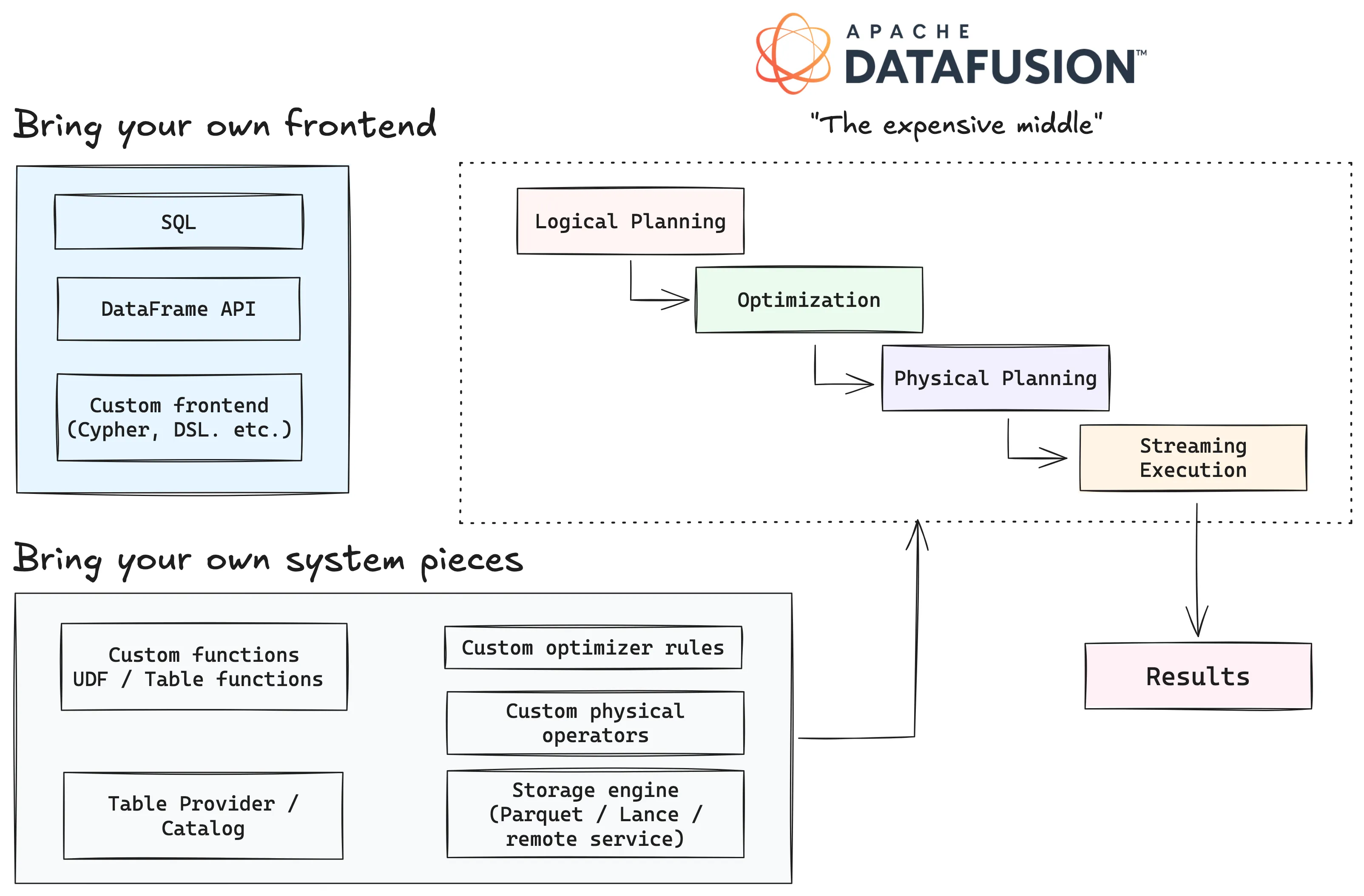
That’s changed since the arrival of Apache DataFusion ⤴: an embeddable, Arrow-native query engine written in Rust that gives systems developers the full pipeline (parsing, logical planning, optimization, physical planning, and streaming execution), without requiring them to build it themselves. It’s becoming the reusable compute layer that sits between a system’s frontend and its storage engine.
This is what enables systems like LanceDB ⤴, Lance-Graph ⤴, and many others to progress at their current pace. Embedding DataFusion’s planning and execution machinery allows engineers to focus their energy on the layers that actually differentiate their systems: storage, indexing, query language, or domain semantics. This post digs into how DataFusion enables all this, why it matters, and why its modular design is enabling a new generation of composable data systems.
What is DataFusion?#
DataFusion is an Arrow-native, embeddable query engine written in Rust 🦀. It’s not a standalone database, because it doesn’t manage its own storage, handle transactions, or ship with a server process. It’s also not “just a SQL parser”. It provides the full pipeline from query to executed results, including parsing, logical planning, optimization, physical planning, and streaming execution over Arrow RecordBatch data.
You can think of DataFusion as a modular collection of pipelines, where each stage provides a hook for different systems to plug into it:
- Frontend: DataFusion ships with both a SQL frontend (built on
sqlparser⤴) and a programmatic DataFrame API. But the frontend is swappable: a system can parse its own language (Cypher, a DSL, etc.) and produce logical plans from it. - Logical planning: The frontend produces a
LogicalPlan: a tree of relational operators (scans, filters, projections, joins, aggregations) that describes what the query computes without specifying how. - Optimization: A chain of
OptimizerRulepasses rewrites the logical plan. DataFusion ships with a substantial set ⤴ out of the box — filter pushdown, projection pushdown, join reordering, common subexpression elimination, and more — but systems can add their own rules or disable built-in ones. - Physical planning: The optimized logical plan gets lowered into an
ExecutionPlan: a tree of concrete operators that know how to produce data. This is where decisions about partitioning, parallelism, and sort order get made. - Execution: Each
ExecutionPlannode implements a pull-based streaming model. Callingnext().awaiton the stream yields ArrowRecordBatchresults incrementally, so even large result sets don’t need to materialize fully in memory.
The result is that DataFusion gives you the expensive “middle of a data system” — the planner, optimizer, and executor — while leaving the edges open. You bring your own storage, your own frontend if you need one, and your own specialized operators. The engine takes care of the relational machinery in between.
A quick look in Python#
The easiest way to see this pipeline in action is through DataFusion’s Python bindings ⤴. The central object is a SessionContext: it holds registered tables, configuration, and the planning/execution machinery.
from datafusion import SessionContext

ctx = SessionContext()

# Register a Parquet file as a table
ctx.register_parquet("trips", "yellow_tripdata_2024-01.parquet")

# Run a SQL query — this returns a DataFrame (lazy, not yet executed)
df = ctx.sql("""
    SELECT
        "PULocationID",
        COUNT(*) AS num_trips,
        ROUND(AVG(trip_distance), 2) AS avg_distance
    FROM trips
    WHERE trip_distance > 0
    GROUP BY "PULocationID"
    ORDER BY num_trips DESC
    LIMIT 10
""")

df.show()
It’s also interesting to see what happens inside that call. We can ask DataFusion to show us the query plan by calling df.explain():
Sort: num_trips DESC NULLS FIRST, fetch=10
  Projection: trips.PULocationID, count(*) AS num_trips, round(avg(trips.trip_distance), 2) AS avg_distance
    Aggregate: groupBy=[[trips.PULocationID]], aggr=[[count(*), avg(trips.trip_distance)]]
      Filter: trips.trip_distance > Float64(0)
        TableScan: trips projection=[PULocationID, trip_distance]
SortPreservingMergeExec: [num_trips@1 DESC], fetch=10
SortExec: TopK(fetch=10), expr=[num_trips@1 DESC], preserve_partitioning=[true]
ProjectionExec: expr=[PULocationID@0, count(*)@1 as num_trips, round(avg(trips.trip_distance)@2, 2) as avg_distance]
AggregateExec: mode=FinalPartitioned, gby=[PULocationID@0 as PULocationID], aggr=[count(*), avg(trips.trip_distance)]
CoalesceBatchesExec: target_batch_size=8192
RepartitionExec: partitioning=Hash([PULocationID@0], 12), input_partitions=12
AggregateExec: mode=Partial, gby=[PULocationID@0 as PULocationID], aggr=[count(*), avg(trips.trip_distance)]
CoalesceBatchesExec: target_batch_size=8192
FilterExec: trip_distance@1 > 0
RepartitionExec: partitioning=RoundRobinBatch(12), input_partitions=1
DataSourceExec: file_groups={1 group: [[trips.parquet]]}, projection=[PULocationID, trip_distance], predicate=trip_distance > 0If you’ve ever looked at an EXPLAIN plan from DuckDB or Postgres, this should look familiar: projection pushdown, predicate pushdown, partitioned aggregation, TopK sort. These are the same operations you’d expect from any mature query engine, coming from an embeddable library.
Observations from the wild#
The DataFusion SIGMOD paper ⤴ describes the shift toward shared, embeddable query engines as the rise of the deconstructed database: modular, reusable components rather than tightly integrated monoliths. This is distinct from embeddable databases like DuckDB, which are excellent tools but still tightly coupled systems — you get the whole package (storage, optimizer, executor) or nothing. DataFusion lets you pick the pieces you need and swap the rest. And the idea now reaches well beyond classic databases — here are just a few examples:
- LanceDB ⤴ embeds DataFusion as its query layer over Lance-backed multimodal data.
- lance-graph ⤴ uses it to plan and execute Cypher queries over the same storage.
- Arroyo ⤴ (now part of Cloudflare) rebuilt its SQL engine around Arrow and DataFusion for streaming compute.
- Apache DataFusion Comet ⤴ uses it to accelerate Spark workloads without changing the user-facing Spark experience.
All these are very different data systems that solve very different problems — yet they’ve all converged on the same reusable query engine under the hood. The reason they can do this is that DataFusion is composable at exactly the right seams.
The interfaces that make DataFusion composable#
The pipeline we saw in the EXPLAIN output above has well-defined boundaries between each stage, and at each boundary there’s an interface (called a trait in Rust) where a downstream system can plug its own logic into DataFusion’s. Let’s walk through the ones that matter most.
TableProvider: teaching DataFusion about your storage#
The most common extension point is TableProvider ⤴. This is how a storage engine tells DataFusion “here’s a table you can query.” The snippet below is in Rust. The TableProvider trait has a small surface area, and the core of it looks like this:
pub trait TableProvider: Send + Sync {
    /// The schema of this table
    fn schema(&self) -> SchemaRef;

    /// The type of table (base table, view, or temporary)
    fn table_type(&self) -> TableType;

    /// Create an ExecutionPlan that reads from this table,
    /// applying projections, filters, and limits where possible
    async fn scan(
        &self,
        state: &dyn Session,
        projection: Option<&Vec<usize>>,  // which columns to read
        filters: &[Expr],                 // predicates to push down
        limit: Option<usize>,             // max rows to return
    ) -> Result<Arc<dyn ExecutionPlan>>;   // returns a node in the physical plan tree

    /// Which filters can this provider handle during scan?
    fn supports_filters_pushdown(
        &self,
        filters: &[&Expr],                // candidate filter expressions
    ) -> Result<Vec<TableProviderFilterPushDown>>; // exact, inexact, or unsupported
}
The key method is scan(). When DataFusion’s planner reaches a table scan node, it calls scan() on the provider with the projected columns, any filter expressions it wants to push down, and an optional row limit. The provider returns an ExecutionPlan (i.e., a node in the physical plan tree) that knows how to produce Arrow RecordBatch streams from whatever storage backs that table.
This is the seam where Lance, for example, connects to DataFusion. Lance implements TableProvider ⤴ so that a Lance dataset looks like any other table to the planner. The optimizer can push projections and filters down through that boundary, and the Lance scan can use its own indexes and fragment structure to serve them efficiently.
Custom functions: extending the expression layer#
Not every extension happens at the plan level. Sometimes you just need DataFusion to understand a new function — a domain-specific scalar, an aggregation, or a window function. DataFusion supports user-defined functions (UDFs) ⤴ that can be registered at runtime and used in SQL or the DataFrame API like any built-in function.
Here’s a small example in Python. Say you want to implement a scalar UDF that clamps a user’s trip distances to a maximum of 10.0. We can write a DataFusion UDF that takes an Arrow array of distances, applies the clamping logic using Arrow compute functions, and returns a new array. Once registered, this function can be used directly in SQL queries.
import pyarrow as pa
import pyarrow.compute as pc
from datafusion import SessionContext, udf

def clamp_distance(distance):
    """Clamp values to a maximum of 10.0"""
    return pc.min_element_wise(distance, 10.0)

clamp_udf = udf(
    clamp_distance,
    input_types=[pa.float64()],
    return_type=pa.float64(),
    volatility="immutable",
    name="clamp_distance",
)

ctx = SessionContext()
ctx.register_udf(clamp_udf)
ctx.register_parquet("trips", "yellow_tripdata_2024-01.parquet")

df = ctx.sql("""
    SELECT
        "PULocationID",
        trip_distance,
        clamp_distance(trip_distance) AS clamped
    FROM trips
    WHERE trip_distance > 8.0
    LIMIT 5
""")
df.show()
+--------------+---------------+---------+
| PULocationID | trip_distance | clamped |
+--------------+---------------+---------+
| 76 | 9.5 | 9.5 |
| 97 | 9.65 | 9.65 |
| 214 | 9.05 | 9.05 |
| 221 | 11.41 | 10.0 |
| 88 | 20.26 | 10.0 |
+--------------+---------------+---------+This is how systems like LanceDB expose domain-specific operations (e.g., vector distance functions) that feel native in SQL queries without forking the engine and rebuilding large parts of it.
Optimizer rules: rewriting plans to fit your system#
DataFusion ships with a substantial set of optimizer rules ⤴ — filter pushdown, projection pushdown, join reordering, common subexpression elimination, and more. But the optimizer is also open. A system can add its own OptimizerRule to rewrite logical plans, or its own PhysicalOptimizerRule to rewrite execution plans.
This matters when a system has knowledge the default optimizer doesn’t. For example, a storage engine that maintains sorted indexes could add an optimizer rule that eliminates unnecessary sort nodes when the data is already in the right order. A graph query system might add rules that fuse certain patterns of joins and filters into specialized graph traversal operators. The optimizer doesn’t need to know about these optimizations in advance — it just needs to run the rules in sequence and let each one inspect and rewrite the plan.
Custom frontends: bringing your own query language#
One of the most powerful aspects of DataFusion that’s easy to overlook is that you don’t have to use SQL at all! DataFusion’s SQL frontend is just one way to produce a LogicalPlan. A system can parse any relevant query language — e.g., Cypher, or a custom DSL over a REST API — and construct logical plan nodes directly. The planner, optimizer, and executor work the same way regardless of where the plan came from.
This is exactly how lance-graph ⤴ (a graph query engine built on top of Lance) works: it parses Cypher queries and lowers them into DataFusion logical plans, then lets the standard optimizer and executor handle the rest. The key point here is that DataFusion doesn’t care about the query language. As long as you can produce a logical plan, you can use the engine.
The bigger picture#
What makes these extension points powerful isn’t any single one in isolation — it’s that they compose. A system can bring its own storage (TableProvider), its own functions (UDFs), its own optimizer rules, and its own frontend, all plugged into the same engine. The relational machinery: scans, filters, joins, aggregations, expression evaluation, memory management — all come for free. The system only needs to build the parts that make it different.
LanceDB: from storage layer to multimodal lakehouse#
LanceDB ⤴ is a good example of what this looks like in practice. It doesn’t just call DataFusion to run the occasional SQL query — it builds its entire SQL execution path on top of it:
- Catalog integration — LanceDB databases and tables are exposed to DataFusion through custom catalog and schema providers. When you write a SQL query against a LanceDB table, the planner resolves table references through these providers and gets back
TableProviderimplementations backed by Lance datasets. From DataFusion’s perspective, it’s just another table it can plan over. - Custom UDFs — LanceDB registers domain-specific scalar functions directly into the DataFusion
SessionContext: distance functions (l2,cosine,dot,hamming) for vector similarity and utility functions likerandom_vectorfor generating test data. These show up in SQL as first-class functions alongside built-ins. - Table-valued functions — Full-text search is exposed as a table-valued function (
fts), so it can be composed with standard SQL filtering and joins in the same query plan. - Custom plan nodes — Operations like
INSERT,UPDATE,DELETE, andCREATE INDEXare implemented as custom logical plan nodes (via DataFusion’sUserDefinedLogicalNodeCoretrait), so they flow through the same planning pipeline asSELECTqueries. - Physical optimizer rules — In LanceDB Enterprise’s distributed deployment, custom
PhysicalOptimizerRuleimplementations rewrite the execution plan to push scans, vector searches, and filtered reads to remote executor nodes — turning a single-node plan into a distributed one without changing the logical query.
One of the most tangible payoffs of building on DataFusion is LanceDB Enterprise’s SQL endpoint ⤴. It exposes a FlightSQL ⤴-compatible interface (i.e., the Arrow ecosystem’s standard wire protocol for SQL-over-Flight), so any FlightSQL client can connect and run analytical queries. In Python, that’s as simple as:
from flightsql import FlightSQLClient

client = FlightSQLClient(
    host="your-lancedb-enterprise-endpoint",
    port=10025,
    token="your-database-token",
    metadata={"database": "your-project-slug"},
)

info = client.execute("SELECT count(*) FROM my_table WHERE category = 'electronics'")
reader = client.do_get(info.endpoints[0].ticket)
table = reader.read_all()
Under the hood, it’s DataFusion that parses the SQL, plans it, optimizes it, and executes it against Lance-backed tables, with all of the custom UDFs, catalog integration, and physical optimizer rules described above. FlightSQL handles the transport. The LanceDB team didn’t need to build a custom query engine or a wire protocol: all it took was composing together existing infrastructure while focusing the real effort on parts that are unique to LanceDB: multimodal storage, vector indexing, full-text search, and distributed execution.
Lance-Graph: same engine, different language#
Here’s an interesting question: what if the query language you’re working with isn’t SQL? A path traversal query like “friends of friends of X who also bought Y” turns into a chain of self-joins, one per hop, and the SQL gets harder to read with every additional step.
Cypher ⤴ is a declarative query language for graphs that expresses the same shape with patterns like (a)-[:KNOWS]->(b)-[:KNOWS]->(c). This isn’t an argument that Cypher is better than SQL — it’s that the frontend is the right place to handle that ergonomic difference. DataFusion’s modular design allows for this level of flexibility without rebuilding the whole engine.
lance-graph ⤴ is a Cypher-capable graph query engine that runs on top of Lance-backed node and relationship tables. Here’s a simple traversal that finds people over the age of 30 and the friends they know:
MATCH (a:Person)-[:KNOWS]->(b:Person)
WHERE a.age > 30
RETURN a.name, b.name
Inside lance-graph, this query goes through four stages before any data gets touched:
- Parsing — a nom ⤴-based Cypher parser (
parser.rs) produces aCypherQueryAST. - Graph logical plan — a
LogicalPlanner(logical_plan.rs) lowers the AST into a graph-aware operator tree, with variants likeScanByLabel,Expand(single-hop traversal), andVariableLengthExpand(multi-hop, e.g.*1..3). - Relational translation — a
DataFusionPlanner(datafusion_planner/mod.rs) rewrites each graph operator into a standard DataFusionLogicalPlan. AnExpandbecomes a chain of joins between the source-node table, the relationship table, and the target-node table. AVariableLengthExpandis unrolled into aUNION ALLof fixed-length expansions, one branch per hop count. - Optimization & execution — from this point on, it’s just DataFusion. Filter pushdown, join reordering, projection pushdown, partitioned execution — all of it works exactly as it did in the SQL example earlier in the post.
By the time the plan reaches DataFusion’s optimizer, it looks like any other SQL logical plan. In fact, the Cypher query above is structurally equivalent to this SQL:
SELECT a.name, b.name
FROM person AS a
JOIN knows  AS r ON a.person_id   = r.src_person_id
JOIN person AS b ON r.dst_person_id = b.person_id
WHERE a.age > 30
DataFusion plans and executes joins over Lance tables, completely agnostic to whether it’s serving a SQL or a Cypher query. Node and relationship tables are just Lance tables behind a thin catalog interface — the graph layer doesn’t own the storage layer, just like the SQL layer doesn’t.
What’s also worth emphasizing is what the lance-graph maintainers didn’t have to build. There are no custom physical operators for graph traversal and no custom optimizer rules to write from scratch. The entire graph engine is essentially a frontend (Cypher parser + graph intermediate representation) plus a lowering pass into standard relational operators. Everything from the logical plan onward is reused from DataFusion.
This is the deconstructed data system thesis playing out in practice: a small team can ship a graph query engine without rebuilding a relational or graph core from scratch, while inheriting every optimizer improvement DataFusion gets for free.
What this means for database builders#
The patterns described above apply to a much larger ecosystem. Once you start looking, DataFusion shows up under the hood in a surprising number of very different systems:
- InfluxDB 3.0 ⤴ rebuilt its time-series storage engine (IOx) on top of Arrow, Parquet, and DataFusion. The user-facing product is still a time-series database, but the query engine is the same one that powers everything else in this post.
- Apache DataFusion Comet ⤴ plugs DataFusion into Apache Spark as a native execution backend. Spark users keep their existing PySpark or Scala code, but operators that Comet can handle get pushed down into DataFusion’s Arrow-native executor instead of the JVM, often with large speedups.
- Arroyo ⤴ is a streaming SQL engine that rebuilt its query layer around Arrow and DataFusion. The semantics are stream-oriented (windows, watermarks, incremental state), but the relational machinery underneath comes from the same library.
- ParadeDB ⤴ embeds DataFusion inside a PostgreSQL extension to bring fast analytical queries over Parquet and Iceberg into a Postgres process, alongside Postgres’s own row-oriented engine.
- Pydantic Logfire ⤴ is an observability platform for LLM and agent applications that ingests traces and logs via OpenTelemetry, stores them as Parquet on object storage, and exposes everything through a SQL Explorer ⤴ backed by DataFusion. The SQL surface is PostgreSQL-compatible, so users (and coding agents) can ask structured questions across spans, logs, and metrics without being boxed into predefined dashboards.
These aren’t toy projects. They’re production systems used in vastly different domains — time series, streaming, distributed batch, OLTP-adjacent analytics, lightweight data APIs — yet they’ve all converged on the same reusable query engine while offering real value in their own domains.
The DataFusion SIGMOD paper ⤴ explains how it can power a “Cambrian explosion” of data systems. That framing feels right: once the cost of building a credible query engine drops by an order of magnitude, the kinds of systems that become economically viable to build also expand by an order of magnitude.
The takeaway for anyone building a new data system is fairly direct. You don’t need to reimplement scans, filtering, projections, joins, aggregations, sorting, or expression evaluation. You don’t need to reinvent an optimizer or write a parallel execution engine from scratch. Those are the parts of a query engine that are hardest to get right and least likely to be the reason a particular product wins. What you do need to focus on is the layer where your system is actually different.
Conclusions#
The data ecosystem has spent the last decade (or more) learning to standardize around reusable formats and protocols — Arrow for in-memory data, Parquet and Lance for on-disk storage, Flight for transport. DataFusion represents the next layer of that same shift: a reusable query engine that systems can embed instead of building from scratch.
Andrew Lamb ⤴ (DataFusion’s most prolific maintainer) describes an FDAP stack ⤴ — Flight, DataFusion, Arrow, and Parquet — as the open foundation for modern analytical systems. For AI and multimodal workloads, Lance slots naturally into that same architecture in place of Parquet, bringing its own advantages around versioning, mixed-type columns, and efficient random access. An FDAL stack — Flight, DataFusion, Arrow, and Lance — is the foundation that both LanceDB and lance-graph are already building on.
The cost of building composable data systems that perform on par with preexisting monolithic systems has dropped sharply. A small team of open source maintainers can now ship a credible storage engine, query language, or domain-specific database without first reinventing the relational core, and the systems they build all benefit from the same compounding improvements happening upstream.
That’s it for this post. The next post will explore lance-graph ⤴ more deeply and dig into its design and performance features, with benchmarks. It’s exciting to imagine what graph query engines built on modular, reusable stacks might look like! 🚀