How Lance enables the Multimodal Lakehouse

Although I’ve been a long-time user of LanceDB ⤴, I hadn’t fully appreciated what was happening under the hood until I began studying it more deeply. LanceDB, and many other platforms at several major companies, are built on Lance ⤴: a modern, multimodal lakehouse format designed from the ground up for AI workloads. Disclaimer: Because I now work at LanceDB, the company, so I’ve got ample time to study the format and its internals on a daily basis. 😁

Anyone who’s worked with data knows that the typical AI workload starts as messy, multimodal raw inputs — text, metadata, images, audio/video. Over time, these get repeatedly enriched with labels, OCR/captions, embeddings, and derived features as the models and the developer’s understanding of the domain evolve. The storage layer has to keep up with schemas that change, tables whose rows and columns drastically grow with time, and workloads that vary from bulk sequential scans to random access (search). These were the challenges that Lance was designed to solve.

When it comes to the Lance ecosystem, there are quite a lot of pieces that come together to form a cohesive whole, so if you’re curious about how Lance works under the hood, how it differs from LanceDB, and when to use each, this post is for you!

Some observations from the wild#

If you look at Lance’s adoption across the industry, you begin to see the same pattern show up across very different teams: frontier labs building multimodal training pipelines, platforms like Netflix’s media data lake ⤴, Uber’s distributed multimodal AI data lake ⤴, and next-generation search engines like Exa ⤴ building data pipelines on top of Lance that can operate at petabyte scale. Although each organization’s use cases may differ, at their core, the storage requirements converge on the same need: a single, scalable data foundation for evolving, multimodal tables that can support mixed workloads.

That “mixed” part is where many lakehouses built around Parquet start to force tradeoffs — they excel at sequential scans, which are the bread-and-butter of analytics. But AI workloads — like training data preparation or agentic search — frequently need both high-throughput scans and targeted seeks (random access) across the same dataset. These needs show up during training shuffles, payload fetches, feature backfills, retrieval, and evaluation. If you pick one access pattern to optimize for, you often pay for it elsewhere via read or write amplification, or operational complexity.

With that context in mind, let’s dive into the design of Lance and how it enables the multimodal lakehouse.

What is Lance?#

Lance is a lakehouse format for multimodal AI. The term “format” can mean a lot of things, so it helps to be explicit: Lance is simultaneously three things: it’s a file format, a table format, and a lightweight catalog spec. We’ll cover each of them in this post.

The first part is the file format: how values become bytes on disk, and how those bytes get turned back into usable types efficiently. On top of that is the table format, providing versioning, data evolution, and indexes that stay consistent with the snapshot readers see. Finally there’s a lightweight namespace spec that makes Lance tables discoverable inside the catalog and compute ecosystem.

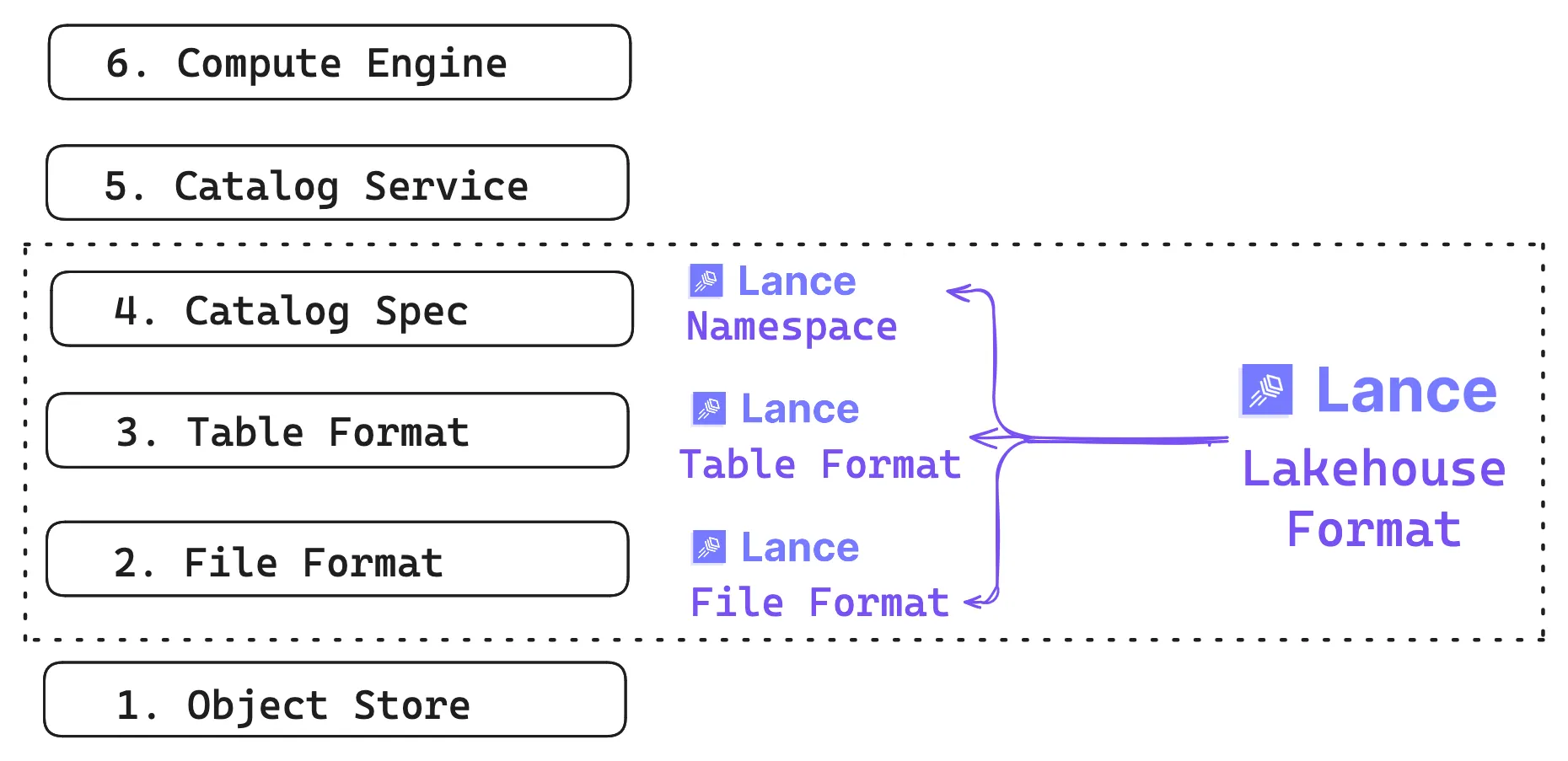
The layers of the modern lakehouse stack

The foundation is still the object store, where Lance datasets typically live (though local disk works too). The same underlying data can be discovered by multiple catalog services and read by multiple compute engines, even when those engines have very different expectations about access patterns.

Primary Design Goals#

As organizations accumulate more and more human- and AI-generated data, the storage layer needs to keep up with a dataset that grows in two dimensions — more rows and more columns. Both the schema and the data continually evolve, adding traditional tabular data and wide fields (blobs). Over time, the system gets hammered by workloads that look nothing alike.

To address these challenges in one format, Lance is designed with the following goals:

Multimodal as first-class: Mixed-width data is considered the norm, from scalars (numbers, strings) to wide blobs (images, audio, video) and embeddings stored next to the metadata in one place.
Data evolution without write amplification: Adding new derived columns writes only the new column values, without needing to rewrite the full table. This makes augmentation and backfills practical as datasets scale.
Fast scans and fast random access: One dataset should handle both throughput-oriented scans and targeted seeks, so training, retrieval, and analytics workloads don’t require the data to live in separate storage systems.
Native indexes: Indexes should live with the data and be versioned alongside it, so everything stays consistent with the snapshot you query.

Before diving into the format internals, it helps to see what working with Lance actually looks like in practice. The core abstraction at the table layer is a dataset: a versioned collection of fragments and indexes that lives at a single location (a directory on disk, or a prefix in object storage). There are two main entry points: pylance (the Lance format library) gives you direct access to datasets, while lancedb (the lakehouse layer) adds a catalog on top, organizing datasets into named tables with search and query capabilities.

`pylance`: Working directly with the Lance format#

The pylance ⤴ library gives you direct, file-level access to Lance datasets. You write and read Arrow tables to disk, manage versions, and control the physical layout. Think of it as the Lance equivalent of writing Parquet files with PyArrow.

import lance
import pyarrow as pa

data = pa.table({
    "id": [1, 2, 3],
    "text": ["cat on a mat", "dog in a fog", "bird on a wire"],
    "embedding": [[0.1, 0.2, 0.3], [0.4, 0.5, 0.6], [0.7, 0.8, 0.9]],
})
ds = lance.write_dataset(data, "./my_data.lance")
print(ds.schema)

`lancedb`: The lakehouse layer#

lancedb ⤴ sits on top of the Lance format and adds lakehouse semantics: named tables, vector search, and a query interface. Under the hood it’s still Lance files, but you interact with them through a higher-level API.

import lancedb

db = lancedb.connect("./my_lakedb")
table = db.create_table("items", data=[
    {"id": 1, "text": "cat on a mat", "embedding": [0.1, 0.2, 0.3]},
    {"id": 2, "text": "dog in a fog", "embedding": [0.4, 0.5, 0.6]},
])
# Vector search is a LanceDB feature, not a format-level one
results = table.search([0.1, 0.2, 0.3]).limit(5).to_polars()

The rest of this post unpacks the format details that make all of this possible, then returns to LanceDB at the platform layer.

Lance file format#

The file format provides the spec for defining containers to store data on disk and the encoding strategy used. Data files store the actual data on disk, and deletion files (a.k.a. deletion vectors) are used to mark rows as deleted without rewriting data files.

Lance files are immutable. Each write operation creates a new version of the dataset. Rather than rewriting the files, rows are removed by marking them as deleted in the deletion files. This approach is faster and avoids invalidating any indexes that reference the files, ensuring that subsequent read queries do not return deleted rows.

Data files#

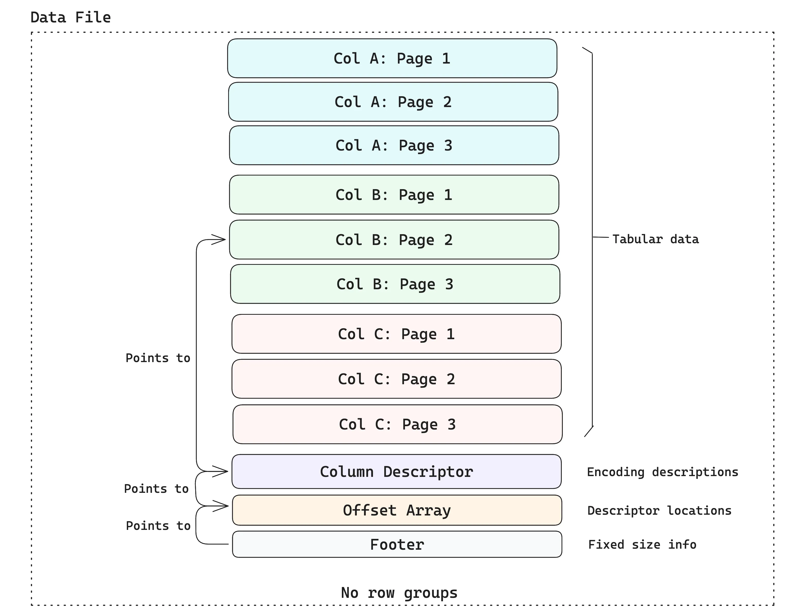
Data files are containers for tabular data. The data is stored in disk pages, where each disk page contains some rows for a single column (the typical page size in Lance is ~8MB). A data file contains multiple pages and may hold data from several columns. The example below shows a data file that holds three columns, each with three pages.

Leveraging Arrow’s type system#

The container format described above has no concept of types, which helps keep the format lean and simple. Instead, Lance leverages Apache Arrow’s type system¹ as far as possible, including both the data type and the encoding (i.e., how the semantic interpretation of data is mapped to the physical layout on disk).

No row groups#

Unlike Parquet, Lance explicitly avoids the use of row groups at the file format layer, as they are detrimental to performance ⤴ when dealing with multiple I/O access patterns. If the row group size is too small, then columns will be split into “runt pages²”, which yield poor read performance on cloud storage. If the row group size is too large, then a file writer will need a large amount of RAM, since an entire row group must be buffered in memory before it can be written.

Instead, Lance splits the file at arbitrary row boundaries and relies on the fact that partial page reads are possible by reading the offset array (see the diagram above) and calculating exactly where to read the page based on the offset. This avoids read amplification while retaining all the benefits of columnar storage.

In practice, this means you can efficiently fetch arbitrary rows by index without scanning the entire dataset:

import lance

ds = lance.dataset("./my_data.lance")
# Fetch specific rows by index -- no full scan needed
rows = ds.take([0, 42, 999])

Adaptive structural encodings#

Once you understand that files are “just pages of bytes,” the next question becomes: how do we store an in-memory array as bytes on disk, and later turn those bytes back into values efficiently at read-time? This is done via encodings.

Lance normalizes Arrow arrays into consistent layouts, then applies an encoding that packs the resulting sequence of bytes (i.e., “buffers”) into a disk page. This matters because the encoding largely determines the tradeoff between fast scans (streaming through lots of rows efficiently) and fast point reads (jumping directly to a small set of rows with minimal extra I/O and decoding).

As stated in the paper ⤴, Lance doesn’t fix one “best” layout for every column, because the right choice depends on the shape of the data (nulls/nesting/variable-width) and the width of values. For wide values (like embeddings, tensors, large strings/blobs), Lance prefers a structure that makes random access predictable — so fetching a specific row doesn’t require chasing multiple side buffers or decoding lots of unrelated data.

For narrow values (like numbers and small strings), Lance favors a chunked, scan-friendly structure that keeps bulk decodes efficient while keeping random access “good enough” (you can decode a small chunk to extract a value).

Lance Table Format#

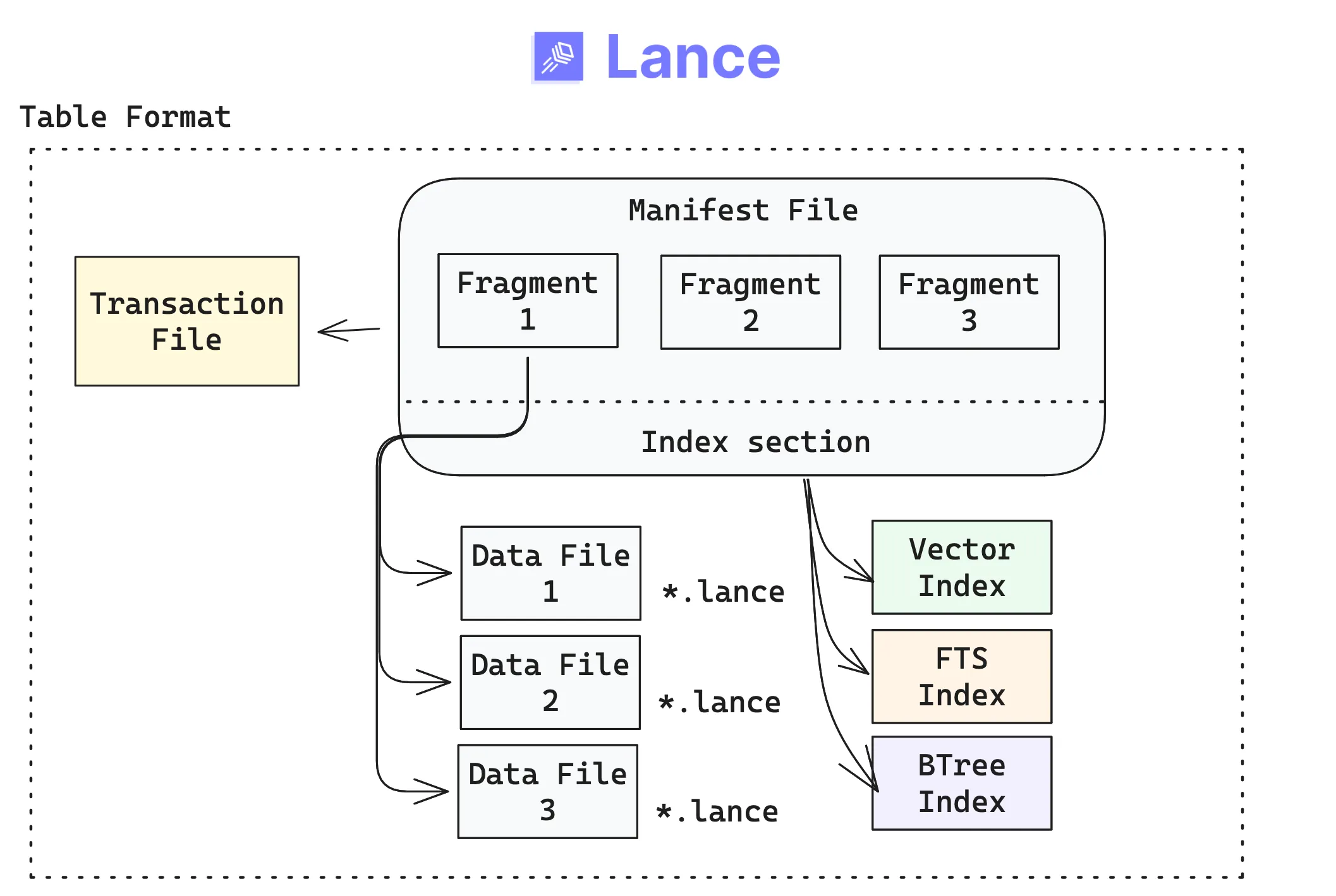
The primary user-facing abstraction in Lance is the table, made up of a few concrete building blocks that live at a physical location (a directory on disk, or a prefix in object storage). If you’ve already worked with other table formats (like Iceberg, Delta Lake, etc.), the design will seem familiar, but with some key differences.The Lance table format organizes datasets as versioned collections of fragments and indexes.

A table version is described by an immutable manifest.
Commits to a table happen via a transaction, tracked in a transaction file. Each transaction creates a new manifest, enabling versioning and time travel.
Fragments are horizontal partitions of data that contain some rows. Fragments are mutable lists in the manifest (they are not files themselves).
Indexes are separate, immutable files referenced by the manifest. Because they’re versioned alongside the table, they stay in sync with the exact snapshot your readers see.

The above components come together at the table layer as follows:

Because each transaction creates a new version, time travel is built into the format. You can always go back to a previous snapshot:

import lance
import pyarrow as pa

ds = lance.write_dataset(pa.table({"id": [1, 2, 3]}), "./versioned.lance")
# Append new data -- creates version 2
lance.write_dataset(pa.table({"id": [4, 5, 6]}), "./versioned.lance", mode="append")
# Read the original version
ds_v1 = lance.dataset("./versioned.lance", version=1)

Two-dimensional storage layout#

Let’s understand how fragments work at the table-level with an example: say you have a product reviews table where you first append new rows. At a later time, you may add new columns that compute derived features (e.g., “sentiment analysis”). The table is growing both vertically and horizontally.

Rows are divided (vertically) into fragments, and fragments are divided (horizontally) into data files. Each data file in a fragment has the same number of rows and contains one or more columns of data.

Adding new rows#

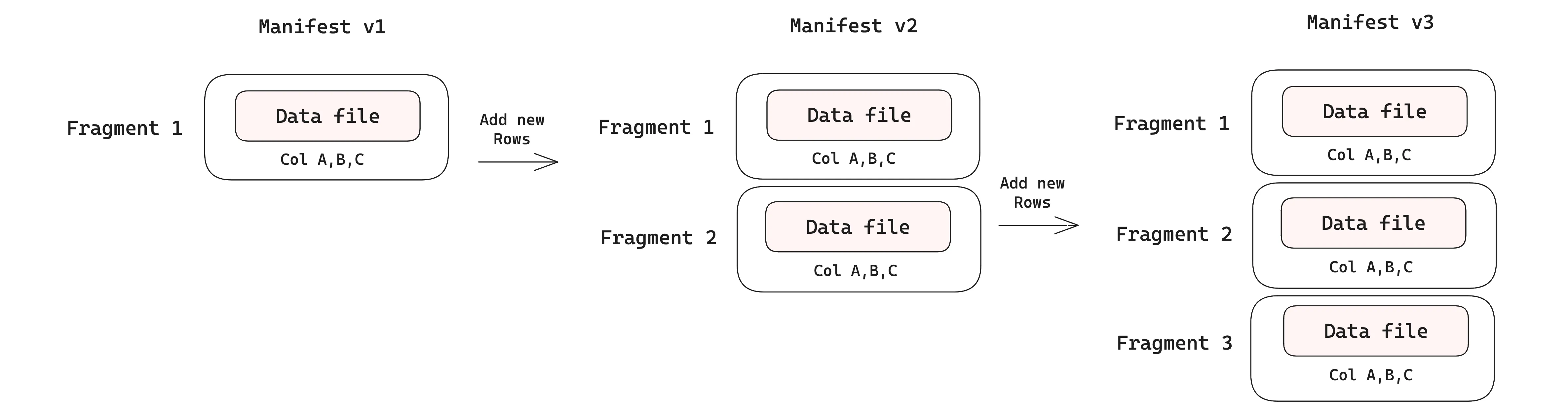
When new rows are appended to a table, each commit creates a new dataset version with its own manifest. In the v1 manifest, we have just a single data file containing the initial rows. Two subsequent appends produce v2 and v3, adding two new fragments, each backed by its own data file. Initially, each fragment is associated with just one data file as only rows are added. The diagram below shows this.

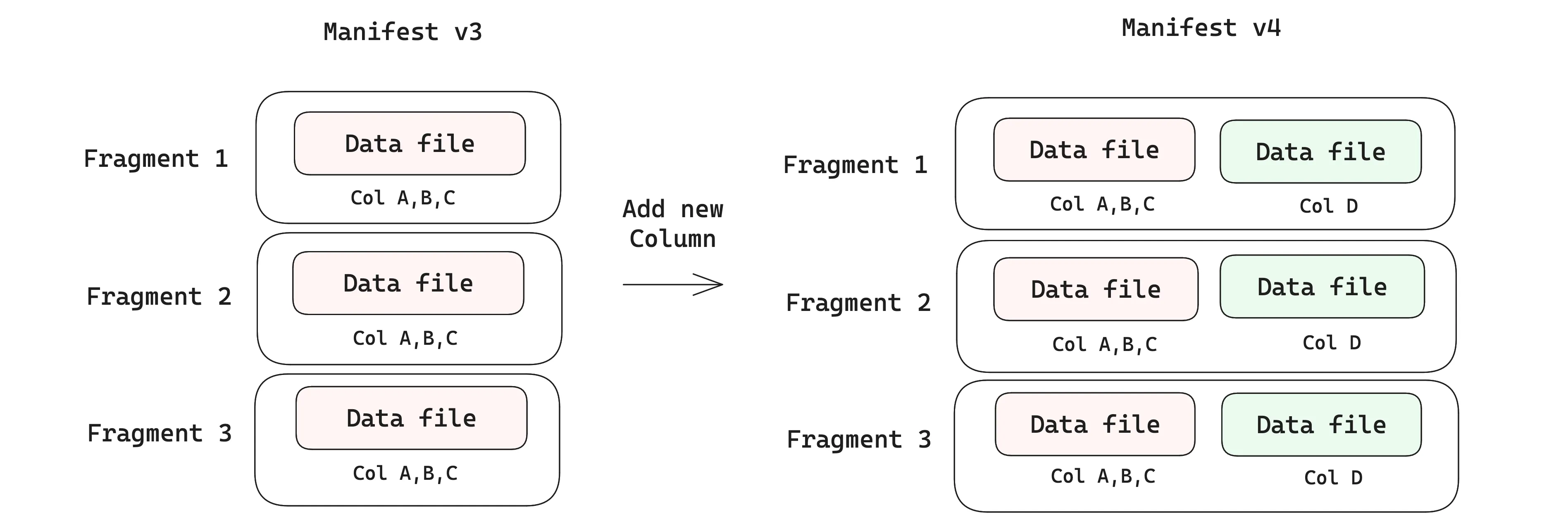
Appending rows to fragments — Appending rows creates a new fragment, each with its own data file

Adding new columns#

Data evolution over new columns is where Lance’s design really shines. Each time you add a new column, a new data file is added to the fragment (keep in mind that fragments are not files — they are just lists in the manifest, so they can be modified). As you add data to the new column, you only write the new data files, while leaving the existing data files untouched. This is fundamentally different from how Parquet-based formats like Iceberg handle schema evolution, where adding a new column requires rewriting the entire file to add the new column’s values, which becomes prohibitively expensive as files grow larger.

Backfilling columns in fragments — Backfilling new columns extends the fragments and does not rewrite existing data. Only the new column's values are written.

Writing only the new data files without rewriting existing data is what lets Lance tables support evolving schemas on very large datasets, avoiding write amplification. In fact, this feature of Lance is key to enabling systems like exa-d ⤴ to update and modify their datasets in production at petabyte scale.

Table management is important in Lance: as the number of fragments grows, it can impact query performance. A compaction ⤴ job is run at regular intervals, which merges fragments and rewrites data files that are smaller than a threshold row count, to keep the number of files reasonable.

Native blob column support#

Multimodal table columns may contain anything from booleans (1 byte) to videos (several GB). In large training datasets, the widest columns are often multimedia blobs, and they tend to dominate the size of the table over time. Without first-class blob support, applications face an uncomfortable choice: either store blobs externally and manage a separate system of pointers, or store them inline and pay the I/O cost of materializing entire payloads even when you only need metadata or a slice.

Lance treats blobs as first-class column types, so they live in the same table as your scalars and embeddings but are stored out-of-line. This means metadata-heavy operations (filtering, joining on scalar columns) never touch the blob bytes, while applications that do need the payload can lazily fetch just the slice they need — a specific byte range of a video, a single frame — without materializing the whole blob in memory. Earlier versions of Lance defined blob columns via schema metadata; starting with file format 2.2, Blob v2 ⤴ introduced dedicated helpers that also support external URI references and byte-range slicing:

import lance
import pyarrow as pa
from lance import blob_field, blob_array, Blob

schema = pa.schema([
    pa.field("id", pa.int64()),
    blob_field("video"),
])

# Store raw bytes directly in the table
inline = b"raw-video-bytes"

# Reference a blob that lives on external storage
external = "s3://bucket/path/video.mp4"

# Reference a byte-range slice of an external blob
slice = Blob.from_uri("s3://bucket/archive.tar", position=4096, size=8192)

blob_values = blob_array([inline, external, slice])
table = pa.table({"id": [1, 2, 3], "video": blob_values}, schema=schema)
ds = lance.write_dataset(table, "./blob_data.lance")

This is what makes Lance practical for multimodal workloads at scale: training data loaders can scan metadata and lazily pull blob batches, multimodal RAG pipelines can search over embeddings without touching video bytes, and exploratory queries can filter first and fetch payloads only for the rows that match.

File-based secondary indexes#

Most formats require you to maintain separate indexes in an external system, which can lead to consistency issues and operational overhead. In Lance, secondary indexes are part of the format itself (e.g., vector, full-text search, and scalar indexes), and are stored as immutable files that are pointed to in the manifest.

An index is a way to speed up data access: instead of scanning the whole table, the engine can look up a value in a column and jump straight to the right rows on disk. Each index in a Lance table is split into segments, where a segment corresponds to a specific set of data fragments. As new data arrives, new segments are added to the index, so queries can combine results from the indexed and unindexed segments until you update the index.

Because indexes are disk-based and managed as part of the table format in Lance, this gives users a very good performance-cost tradeoff compared to other data systems and table formats.

Lance Namespace Spec#

Once you move beyond a single table, you need a way to organize and discover datasets. In enterprise lakehouses, that layer is usually the catalog: the system that names tables, groups them logically, and lets compute engines find the right thing without hard-coding object-store paths.

Lance’s catalog-level abstraction is called the Namespace ⤴. The namespace spec defines a unified model for describing tables and their relationships inside a hierarchy, along with the operations available on those objects. It’s the piece that turns “a directory full of tables” into something you can browse, reason about, and plug into other parts of your stack.

It’s important to understand that LanceDB itself is built on top of the Lance format, and operates at the catalog level, where the first thing you typically do is connect to a lakehouse (which is outside the scope of the table format). LanceDB OSS uses the simplest form of a namespace spec: a single-level directory (typically named data/), under which all tables are stored.

/local_lancedb/  # Root Namespace
└─ users.lance   # Table ["users"]
    └─ data/     # Data files for "users" table
└─ orders.lance  # Table ["orders"]
    └─ data/     # Data files for "orders" table

To generate such a directory structure, it’s just a few lines of code:

import lancedb

db = lancedb.connect("./local_lancedb")

user_data = [{"id": 1, "vector": [0.1, 0.2], "name": "alice"}]
order_data = [{"id": 1, "user_id": 1, "amount": 100}]

table = db.create_table("user", data=user_data, mode="create")
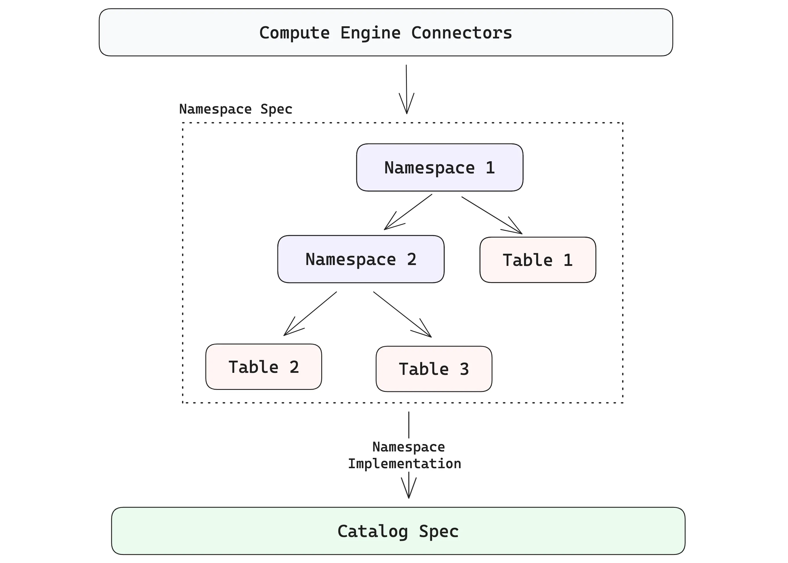
table = db.create_table("orders", data=order_data, mode="create")

Namespaces are generalizations of catalog specs that give platform developers a clean way to present Lance tables in the structures users expect. The diagram below shows how the hierarchy can go beyond a single level. A namespace can contain a collection of tables, and it can also contain namespaces recursively.

Hopefully, it’s easy to see how these pieces come together to enable a lakehouse where multimodal data, indexes and evolving datasets all come with first-class support, rather than being bolted on as an afterthought.

Tying Together These Concepts#

At the file format level, Lance’s page-based layout with offset arrays, lack of row groups, and adaptive structural encodings make fast scans and fast random access possible on the same dataset. Leveraging Arrow’s physical types along with a special large binary encoding makes first-class multimodal support practical: you can efficiently store wide fields alongside narrow metadata without splitting your training set or knowledge base across multiple systems.

At the table format level, versioned manifests and fragments mean that updates are basically “write new files and publish a new version” — this is the key mechanism behind Lance’s flexible data evolution that only writes new data without touching existing data files. Also, because indexes are immutable files referenced by the manifest, they are part of the dataset and its associated version. This means that retrieval, training and analytics can all operate against the same version of the data.

Namespaces are a catalog-level abstraction, making Lance tables discoverable and composable across compute engines and catalog specs that are used elsewhere in the lakehouse ecosystem.

LanceDB and the Multimodal Lakehouse#

Lance (the format) gives you the building blocks: fast scans and random access, immutable files, versioning, and disk-native indexes that scale. This section moves up one layer to LanceDB, the primary developer-facing interface built on top of the format. It starts as an embedded OSS library and extends into a managed data platform when production systems need always-on services and distributed compute.

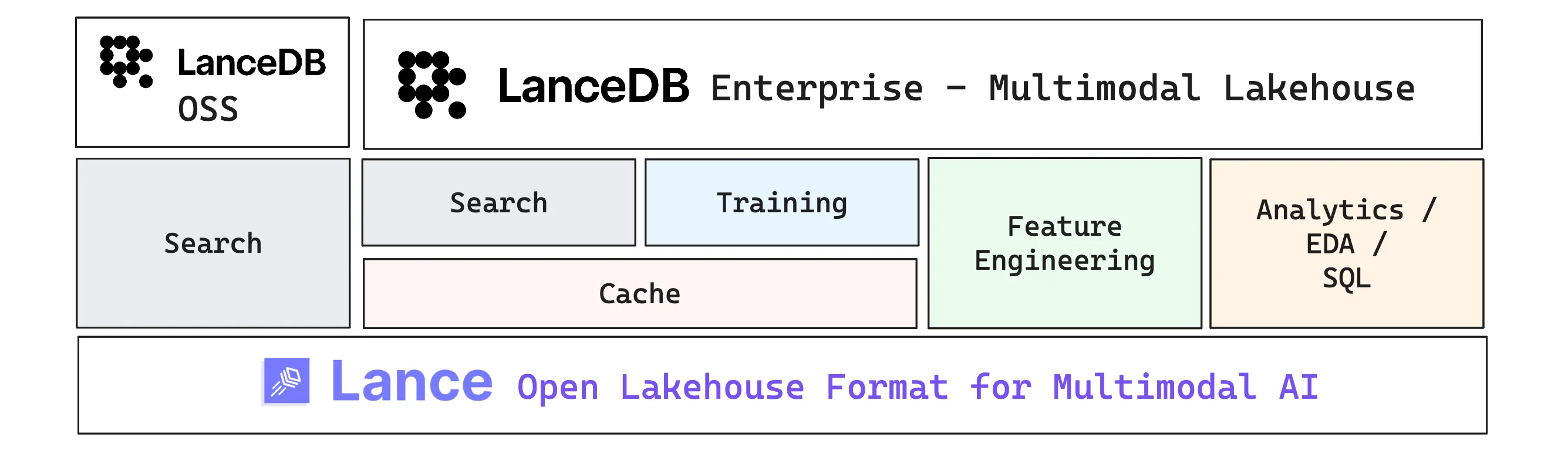
LanceDB is the data management layer built on top of the open source Lance format. LanceDB OSS is an embedded multimodal lakehouse library that can run on your local machine or inside a single application process. LanceDB Enterprise builds on the same foundations and adds the operational layer for production: always-on services and distributed compute that help you scale ingestion, indexing, caching, and feature pipelines. We’ll unpack those Enterprise capabilities in the sections below.

When should you use Lance vs. LanceDB?#

The distinction isn’t about capability — both layers support vector search, versioning, and indexing. It’s about where you sit in the stack and what you want to manage yourself.

If you’re a platform engineer integrating Lance into an existing catalog and compute stack, reach for pylance ⤴. It gives you direct control over datasets, namespaces, and the physical layout — the building blocks for wiring Lance into your own infrastructure. Vector search, for example, works but you’re tuning the knobs yourself:

ds.to_table(
    nearest={
        "column": "vector",
        "q": query_vector,
        "k": 10,
        "nprobes": 10,
        "refine_factor": 5,
    }
).to_pandas()

If you’re an AI/ML engineer building applications — retrieval systems, training pipelines, feature engineering workflows — start with LanceDB ⤴. It wraps the same underlying format into a higher-level interface with table management, a fluent query builder, and automatic handling of the operational details:

results = (
    table.search([0.1, 0.2, 0.3])
    .where("id > 1")
    .limit(5)
    .to_polars()
)

Not that Lance and LanceDB are not competing tools: LanceDB sits on top of Lance. The key difference is that LanceDB gives you a clear path from local experimentation (LanceDB OSS, an embedded library) to production-scale deployment (LanceDB Enterprise, with automatic reindexing, compaction, and distributed compute), so you can focus on your AI workload rather than the infrastructure underneath.

Below, we list some of the reasons why teams are actively choosing to use LanceDB Enterprise for some really hard problems in production.

One system for many workloads³#

AI teams typically end up stitching together multiple systems: a vector DB for retrieval, a warehouse for analytics, and custom infrastructure to manage training data. LanceDB’s goal is to collapse as many of these workloads into one bucket with a convenient SQL interface, so you can do things like:

Training caches to manage large datasets on cloud storage and rapidly experimenting with datasets for training jobs
Semantic retrieval for multimodal RAG (serving text, images, and multimedia to agents)
Exploratory search on petabytes of image/video data and deduplication based on semantic similarity
Interactive exploration (filters, joins, aggregations) on the same tables used for the above tasks

Keeping GPUs fed with a training cache#

Large training jobs can fan out to hundreds of GPUs, and the easiest way to stall them is to have everyone read directly from an object store at once. This can lead to throttling and slow starts, requiring very expensive egress to external “hot tier” systems. A training cache lets you prewarm and serve hot training shards close to compute so GPUs stay utilized and you avoid repeated object-store reads.

This also matters in a multi-cloud/“neocloud” world: you can keep the source of truth in object storage and deploy caches near whichever GPU fleet you’re using, so you get portability without re-architecting your storage layer.

Scalable feature engineering with Geneva#

Once you have raw data, you quickly need derived columns: embeddings, OCR/captions, audio features, thumbnails, quality signals, and model outputs. At scale, it’s not enough to run a one-off batch job. You need a distributed system that can compute and backfill features reliably, repeatedly, and concurrently with reads and writes.

LanceDB Enterprise’s multimodal feature engineering package (Geneva ⤴) helps manage these workloads with provenance and reproducibility baked in. It supports versioned UDFs so your transforms are reproducible: you can trace not only which data version you trained on, but also which transform/version of code produced the features in that table version.

True scalability across the table lifecycle#

Although many training workloads begin with “can I prepare a 100 million row training dataset?”, as you productionize the training pipeline, the question can quickly become “how can I maintain and filter the relevant data on a 100 billion row dataset with text and images to train the next foundation model?” Similar scalability questions also appear in search or analytical workloads.

At petabyte scale, everything is hard. You need distributed ingestion, distributed indexing, distributed shuffles, and careful use of caching so only a small fraction of data needs to be kept hot at any moment. LanceDB Enterprise builds on Lance’s disk-native features to scale index construction (including GPU-accelerated workflows), querying, and training data maintenance across many workers, allowing teams to focus on AI engineering, without getting bogged down by the infrastructure engineering required for production.

Conclusions#

This was a long, but (in my opinion, necessary) post on the design of Lance — from the file format’s page-based layout and adaptive encodings, through the table format’s versioned manifests and fragments, all the way up to LanceDB’s lakehouse and platform layer. The goal was to clarify each level in detail, and when you’d reach for either pylance or lancedb depending on your needs.

At a lower level, pylance gives you control over Lance datasets: random access by row index, vector search, blob encoding for multimodal payloads, built-in versioning that lets you time-travel across snapshots, and the ability to integrate Lance with other parts of the lakehouse stack at the namespace level. At a slightly higher level, lancedb wraps these capabilities into a convenient interface that offers all the features of the underlying format, as well as a fluent query builder and a clear path from embedded local use to production-scale deployment via LanceDB Enterprise.

What’s exciting is that the ideas Lance brings are highly practical, not just theoretical, and are already being used in production in several organizations. To my eyes, Lance’s adoption is growing across the ecosystem because it solves several pain points all at once: keeping large AI datasets evolvable without rewrites, serving training, retrieval, and analytics use cases from the same source of truth, and scaling to sizes where “just scan it” stops being an option.

As enterprise organizations and research labs push toward larger, increasingly multimodal datasets for their training and retrieval needs, the gap between “works on a PoC” and “works at immense scale” keeps widening. Lance is designed to close that gap: build one versioned, multimodal source of truth that can serve training, retrieval, and analytics without splitting your stack. 2026 is shaping up to be the year of the multimodal lakehouse!

If you’ve made it this far, thanks for reading! I hope this post helps clarify the design of Lance and what it can enable for the upcoming era of AI-native data platforms. I fully intend to do more deep-dive explorations like these on other aspects of the Lance ecosystem, as well as how LanceDB is used in real-world applications. Stay tuned for more! 🚀