Learning DSPy (3): Working with optimizers
A walkthrough of using the bootstrap fewshot and GEPA optimizers in DSPy
Welcome back to the Learning DSPy series! So far, we’ve discussed the core building blocks of DSPy (signatures and modules, without going into optimizers), and highlighted the strengths of the programming model offered by DSPy. In this post, we’ll take a closer look at optimizers, and how they can be used to automatically improve the performance of a DSPy program.
To understand the optimization workflow in DSPy, we’ll use the example of the mergers and acquisitions (M&A) module that was discussed in part 1 of this series, where the task was to extract structured information from news articles about M&A events.
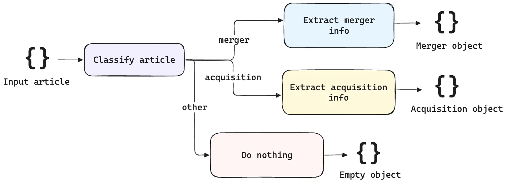
The input is a news article covering a potential M&A event, and the output is a structured JSON object representing information extracted from the articles, such as the acquirer, target, deal value, and so on. Based on the classification step upstream, a different structured output is obtained, depending on whether the event is a merger or an acquisition.
Optimization is more like compilation#
A DSPy program is a collection of one or more modules, composed together for a larger goal and purpose. Each module depends on a signature, which combines code (types) and English (instructions) to define the intent of the program. The M&A example above consists of a compound module that encapsulates three submodules: a classification module, a merger module and an acquisition module, each with their own signatures.
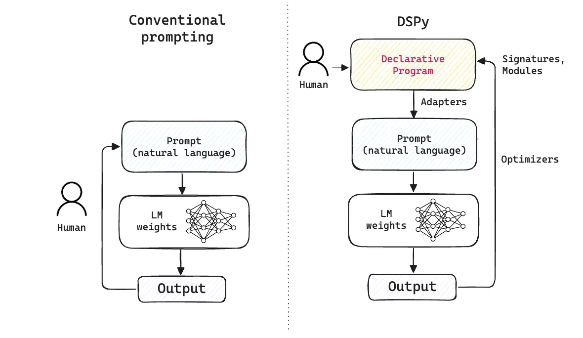
The key point to note here is that DSPy offers a declarative interface for building AI systems, where the prompt is managed by the framework, rather than being hand-crafted by the developer. You can think of the DSPy program as an abstraction over the prompt (that you may be used to writing by hand, if you’re coming from other frameworks), per the following diagram:
If you’re like me, and come from a machine learning background, the term “optimization” might conjure up images of gradient descent, backpropagation, and other techniques commonly used in training neural networks. Before proceeding any further, let’s first throw these ideas out of our heads!
Optimization in DSPy is more akin to the process of compilation in programming languages. The goal of DSPy is to translate high-level instructions (via signatures + modules) to low-level instructions that the LM can work with (i.e., weights). Just like C++ or Rust compilers eventually translate down to assembly code, when we “compile” a DSPy program, we’re doing to the prompt what a compiler does to source code.
Just as we don’t expect the average C++ or Rust developer to wrangle with bytecode or assembly code (we only expect that the user writes source code in that language), DSPy’s optimizers operate on a similar premise — the user writes declarative code in the language of choice (most commonly, Python) without needing to wrangle with prompts or LM weights.
DSPy is a language (an embedded language). It is to prompts what C++ is to assembly.
— DSPy (@DSPyOSS) August 11, 2025
Our job is to "turn DSPy code into Python + prompts + weights". The semantics are partly fuzzy, but it's important to see that the English (signatures) in a DSPy program is written *to be…
For these reasons, optimization is synonymous with “compilation” in the DSPy community. There isn’t one universal way to do optimization in DSPy. Just like there are several compilers for programming languages (e.g., GCC, Clang, Intel … in the case of C++), each of which encode their own heuristics and domain knowledge, there are also several optimizers in DSPy, each of which operate on different parts of the program, with different strategies to improve the outcome.
The surface area of optimizers#
Let’s look at the full prompt that’s generated by a DSPy signature, and understand
which parts of it the optimizer can modify. To display the full prompt, we can use
the dspy.inspect_history(n=3) method. The n=3 argument indicates that we want to see the
results from the last three LM invocations, because we have three submodules in our M&A
information extraction module that each call the LM once for a given news article.
import dspy

# Define the signatures and modules here ...
# Then, instantiate the module
extract = Extract()

text = article["title"] + extract_first_n_sentences(article["content"], 5)
result = extract(text=text, article_id=article_id)
# For debugging, inspect the prompts sent during the last 3 LM calls
print(dspy.inspect_history(n=3))
A DSPy prompt has several parts, as shown below for the classification submodule. The prompts for the merger and acquisition modules are similar in structure, but have different signatures and instructions.
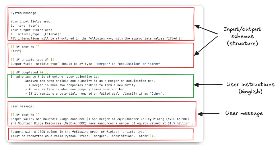
Writing signatures allows developers to combine English (via user instructions) along with code that defines structure (via Pydantic models and signature descriptions), allowing DSPy to then create a prompt that the language model can use to perform the task.
The “surface area of optimization” is the portion of the prompt that the optimizer can target to improve performance on the task. In the diagram above, the green bounding box represents one of these areas, which corresponds to the user instructions. There are two broad ways that optimizers can modify the prompt:
-
Fewshot examples: The optimizer can add, remove or modify fewshot examples from which the model can learn during inference time. This is the easiest and cheapest way to optimize a DSPy program. When adding fewshot examples, the optimizer leaves the entire prompt unchanged — it simply adds demos to the “assistant message” section of the prompt (shown later in this post).
-
User instructions: Certain classes of optimizers (like MIPROv2, SIMBA and GEPA) can rewrite the user instructions in the prompt. This is extremely powerful, because it allows the optimizer to find potentially better instructions than humans might write, because it’s able to algorithmically explore a much larger space to identify the optimal phrasing of the instructions. We’ll look at a few examples of high-quality prompts that GEPA writes, in a moment.
Prerequisites for optimization#
Optimization is an algorithmic process that can tune prompts (and also the LM weights, but that’s outside the scope of this post). Before diving into the details of how it works, it’s worth understanding the prerequisites for optimization:
-
A DSPy program: The program that you want to optimize. It can be a single module or a compound module consisting of multiple submodules (like our M&A information extraction module).
-
Metric: A function that evaluates the output of the DSPy program and returns a score (higher is better).
-
Examples: Anywhere from 10 to a few hundred examples that can be split into train and test sets. Different optimizers have different requirements for the number of examples needed, but for modifying prompts, a few dozen examples is usually sufficient as a starting point.
We already covered the details of the DSPy program in part 1, so we won’t repeat them here. Next, let’s define a metric for evaluating the overall output of the M&A information extraction module.
Recall that the output of the program in this case is a structured output, represented as a JSON object. Some examples of the output are shown below. Note how there are a combination of different data types (strings, numbers, lists) in each output.
{
  "article_id": 13,
  "parent_company": "Titanium Corp",
  "parent_company_ticker": ["TSX:TCP"],
  "child_company": "Azure Mining",
  "child_company_ticker": ["TSX:AZM", "NYSE-A:AZZ"],
  "deal_amount": "4.2 billion",
  "deal_currency": "CAD",
  "article_type": "acquisition"
}
{
"article_id": 18,
"company_1": "Copper Valley Mining",
"company_1_ticker": ["NYSE-A:CVMI"],
"company_2": "Mountain Ridge Resources",
"company_2_ticker": ["NYSE-A:MORR"],
"merged_entity": "Valley Ridge Mining",
"deal_amount": "1.5 billion",
"deal_currency": "USD",
"article_type": "merger"
}{
"article_id": 8,
"article_type": "other"
}Define metric#
The core data type in DSPy is Example, which is used to provide the training data
to the optimizer. The following snippet shows how to construct an example based on the Pydantic
models for “merger”, “acquisition” and “other” types of articles:
def get_pydantic_model(json_data: dict) -> Merger | Acquisition | Other:
    """Reconstruct a Pydantic model from the given JSON object"""
    article_type = json_data.get("article_type")

    if article_type == "merger":
        return Merger(**json_data)
    elif article_type == "acquisition":
        return Acquisition(**json_data)
    else:  # article_type == "other"
        return Other(**json_data)


def create_dspy_examples(num_sentences: int, article_ids: list[int]) -> list[dspy.Example]:
    """Create a list of dspy.Example objects for the given article IDs."""
    examples = []
    for article_id in article_ids:
        article = get_article_by_id(articles[article_id])
        # Input text is the the title + first 5 sentences of the article
        text = (
            article["title"] + "\n" + extract_first_n_sentences(article["content"], num_sentences)
        )

        # Obtain the expected Pydantic model from gold data
        expected_output = get_pydantic_model(get_article_by_id(articles[article_id]))

        # Create dspy.Example with inputs marked
        example = dspy.Example(
            text=text, article_id=article_id, expected_output=expected_output
        ).with_inputs("text", "article_id")
        examples.append(example)
    return examples
We first extract the input text, which is the title + first 5 sentences of the article that provides
context to the LM for the task at hand (classification or information extraction). Next,
we reconstruct the expected outputs from the gold data, and finally, we create
an Example object, marking the input fields using the with_inputs() method. Anything
that’s not marked as an input is assumed to be a label or metadata field.
Next, we need to define a metric function that can compare the predicted output against the expected output. Because this is a structured output task, it’s simple to define an “exact match” score that returns 0.0 if any field is incorrect, and 1.0 if all fields are correct.
def validate_answer(
    example: dspy.Example,
    pred: Merger | Acquisition | Other,
    trace=None,
) -> float:
    """DSPy-compatible metric function for evaluating extraction results."""
    expected = example.expected_output

    # Type mismatch or Other type handling
    if not isinstance(pred, type(expected)):
        return 0.0
    if isinstance(expected, Other):
        return 1.0

    # Compare all model fields using Pydantic's field info
    expected_dict = expected.model_dump()
    pred_dict = pred.model_dump()

    # Calculate field-level accuracy scores
    matches = [metric(expected_dict[field], pred_dict[field]) for field in expected_dict]

    # Return average exact match score across all fields
    return sum(matches) / len(matches) if matches else 0.0
The validate_answer function returns the average exact match score across all fields
in the output, which is the metric that will be maximized during optimization.
The code for the evaluation metric and scoring is available here ⤴.
Define dataset#
The dataset used for optimization is simply a list of Example objects, numbering anywhere from ten
to a few dozen (or hundreds, if available). Unlike optimizing LM weights, which typically requires
thousands of examples and many rollouts, optimizing
prompts can be done with a much smaller number of examples, typically under 100.
For this post, a mix of 34 real + synthetic examples (generated by GPT-5) were used. The dataset
is stored in a gold.json file that contains the human-labelled expected outputs for each article,
and the dataset is then split into train and test sets, similar to how you would do in traditional machine
learning.
The articles are identified by their IDs, and the following code snippet shows how the train
and test sets are defined using the create_dspy_examples function defined above.
# Define IDs for train/test splits and create Examples for training/testing
train_ids = [2, 5, 6, 1, 7, 4, 10, 9, 11, 3, 12, 13, 8, 14]
train_set = create_dspy_examples(num_sentences=5, article_ids=train_ids)

test_ids = [17, 15, 18, 19, 16, 20, 22, 21, 28, 23]
test_set = create_dspy_examples(num_sentences=5, article_ids=test_ids)
Note that the article IDs are not randomly sampled from the gold dataset. Instead, they were hand-picked to ensure a good mix of “merger”, “acquisition” and “other” types of articles for both the train and test sets, for the following reasons:
- It provides the optimizer a stronger signal during training, because it’s able to see a wider variety of article types (rather than being skewed towards one type)
- It ensures a fairer comparison between the test set and the training set (e.g., it would be unfair to train the optimizer on 90% “merger” articles, and then test it on 90% “acquisition” articles!)
Because we don’t need a large number of examples for optimizing prompts in DSPy, it’s relatively trivial to begin optimizing your workflow by hand-picking a few dozen high quality set of examples, and splitting them into train/test sets.
Option 1: Automatic fewshot learning#
The simplest way to optimize a DSPy program is to include fewshot examples (i.e., “demos”) from the provided examples for training. One such approach is called “bootstrap fewshot”, which is available out-of-the-box in DSPy. This approach doesn’t modify the user instructions at all, but rather, appends a few examples to the prompt that improve the context.
Bootstrap fewshot optimization works by mixing (a) some labeled demos with (b) bootstrapped demos that it
generates by running a teacher LM over your train inputs, collecting the teacher’s predictions
(and traces), filtering candidates with the metrics, and keeping the best as demos for the
student. It can iterate for multiple rounds and explicitly bypass caches with a new rollout_id to
diversify results2.
By default, the teacher and the student are the same model, but it’s trivial to specify a more capable model for the teacher, while using a small, cheap model for performing the task.
import dspy

# Choose a more capable model for the teacher
teacher_lm = dspy.LM('google/gemini-2.5-flash')

# Choose a smaller, cheaper model for the student
student_lm = dspy.LM('google/gemini-2.5-flash-lite')
The following snippet shows how to set up bootstrap fewshot optimization with some optional hyperparameters that can be tuned. The teacher model settings are also passed explicitly.
optimizer = dspy.BootstrapFewShot(
    metric=validate_answer,
    max_bootstrapped_demos=4,
    max_labeled_demos=14,
    max_rounds=1,
    max_errors=10,
    teacher_settings={"lm": teacher_lm},
)
In just a few lines of code, DSPy automatically constructs fewshot examples that the student LM can use during inference time, by running the teacher LM over the training inputs.
In this case, we already provide ample examples in the training set (14 examples), which is equal
to the max_labeled_demos parameter, so the optimizer will most likely use all of them, because
they are high-quality and human-labelled. Bootstrapping with a larger number of max_rounds can
potentially help discover better examples, but it also increases the number of LM calls, so
it’s generally a good idea to provide a good set of labelled examples upfront.
The following table shows the improvement in average exact match score on the test set, before and after bootstrap fewshot optimization.
| Case | Average Exact Match Score |
|---|---|
| Baseline | 80.7% |
| Bootstrap Fewshot | 90.7% |
The bootstrap fewshot optimizer was able to improve the program’s performance by 10%!
Let’s look at what actually changed in the prompt sent to the LM, by inspecting the last LM call
via dspy.inspect_history. The system and user instructions remain unchanged — all that’s added
are some new user and assistant messages, corresponding to the fewshot examples that were added
by the optimizer.
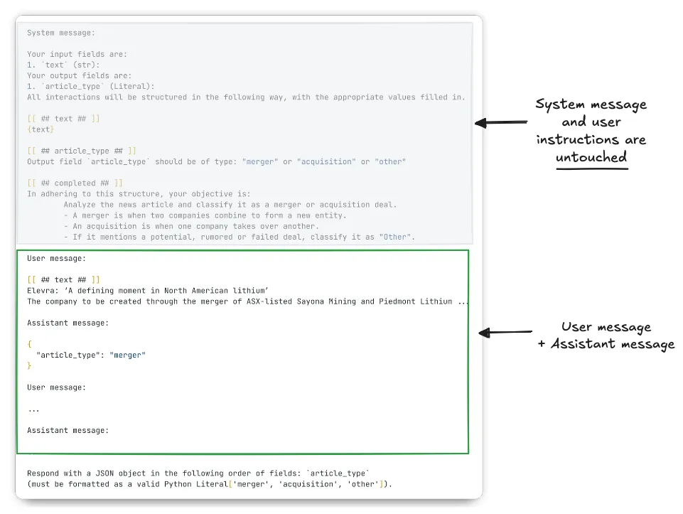
There are 4 demos included via the prompt’s user + assistant message interface
(2 mergers, one acquisition and one “other”). The reason there are 4 examples is that we set
max_bootstrapped_demos=4. Setting this parameter higher will include more demos in the prompt,
which could further improve results (with diminishing returns
beyond a point).
Automatic fewshot optimization is a good initial step to improve the baseline performance of a DSPy program without having to manually craft fewshot examples (you can just use a part of your evaluation dataset) and DSPy will take care of the rest. However, it’s still a rather naive approach, because all it does is add demos to the prompt, without modifying the user instructions at all.
To optimize the user instructions, we need a more advanced optimizer like GEPA. 👇🏼
Option 2: GEPA#
GEPA (GEnetic PAreto optimization) is one of the more exciting developments of the AI landscape in 2025. Introduced by Agrawal et al. in this paper ⤴ in July 2025, GEPA has gained rapid adoption and praise in the DSPy community, because it writes great prompts that often outperform the best human-engineered prompts, while also being highly sample efficient. Below, we’ll see how a dataset of just 34 examples (14 train, 10 validation and 10 test) was able to significantly improve our information extraction pipeline to get up to a score of 97.8% on the test set!
How GEPA works#
A deeper dive into the technical details of GEPA will be reserved for a future post, but in this section, it’s worth understanding the high-level workflow of GEPA, and what it actually does under the hood.
The core premise of GEPA (as stated in the paper ⤴) is that “algorithms that learn deliberately in natural language by reflecting on serialized trajectories of information in natural language, such as the instructions, the reasoning steps, tool calls”, can make much more effective use of the strong language priors that LMs have learned during their training. This explains the sample-efficiency of GEPA compared to reinforcement learning — rather than collapsing the reward signal to a single scalar function (as in RL), the algorithm exploits the biggest strengths of language models, i.e., their ability to generate and reason over natural language. GEPA does this entirely without relying on gradients (unlike RL).
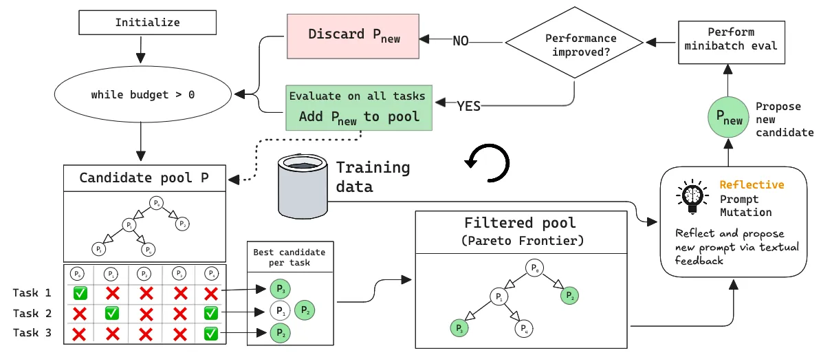
The GEPA workflow begins with initializing a candidate program, with baseline user and system instructions. A training budget (“light”, “medium”, or “heavy”) is specified, which controls the maximum number of rollouts (end-to-end executions of the program) that the GEPA optimizer can use during training. The optimization begins with GEPA proposing new candidate instructions, creating a pool of programs that can be progressively improved through multiple generations. Each stage produces increasingly more effective candidates by modifying existing ones through mutation or crossover, which are standard gradient-free techniques in evolutionary algorithms ⤴.
The GEPA algorithm uses a “reflection LM”, which is a capable language model (e.g., gemini-2.5-pro/gpt-4.1 calibre or better)
to propose new instructions for each candidate. The student LM can be a smaller, cheaper model whose prompt is being
improved based on the new instructions proposed by the reflection LM.
The key innovations in GEPA that make it work so well are:
-
Reflective prompt mutation: GEPA uses an LM to reflect on the execution traces (inputs, outputs, failures, or any other form of feedback) for a given module. It then proposes a new instruction that’s tailored to the specific errors or shortcomings of the previous instruction, based on the feedback.
-
Pareto selection: GEPA maintains a Pareto frontier, which is a collection of the best candidate programs that did well on each task, rather than just the best global candidate. This allows it to rapidly explore the prompt space while also retaining complementary strategies that work well for the overall task.
-
Text as feedback: GEPA can leverage any textual feedback as a learning signal, including logs, error messages, failed parses or code traces, which allows language models to take action with a higher level of domain awareness.
Running GEPA in DSPy#
Because GEPA requires textual feedback for the reflection language model, a new metric function with feedback is needed. The following code snippet shows how to define a metric function that returns both the score and text feedback that GEPA can use to reflect on the program’s performance.
def validate_answer_with_feedback(
    example: dspy.Example,
    pred: Merger | Acquisition | Other,
    trace=None,
    pred_name=None,
    pred_trace=None,
) -> dspy.Prediction:
    """Metric for GEPA that mirrors validate_answer while emitting per-field feedback and score"""
    expected = example.expected_output

    # If incorrectly classified, score is instantly zero
    if not isinstance(pred, type(expected)):
        feedback = f"Article {example.article_id}): expected {type(expected).__name__}, got {type(pred).__name__}"
        return dspy.Prediction(score=0.0, feedback=feedback)

    # If other, no fields to compare, and score is 1.0
    if isinstance(expected, Other):
        feedback = f"✅ Article {example.article_id}): correctly classified as Other"
        return dspy.Prediction(score=1.0, feedback=feedback)

    # If the classification is not "Other", score on all model fields using Pydantic field info
    expected_dict = expected.model_dump()
    pred_dict = pred.model_dump()

    scored_fields = 0
    matches = 0

    feedback = f"Feedback for Article {example.article_id}:\n"
    for field, gold_value in expected_dict.items():
        if field in ["article_id"]:
            continue

        predicted_value = pred_dict.get(field)
        field_score = metric(gold_value, predicted_value)
        scored_fields += 1
        matches += field_score

        if field_score:
            feedback += f"  ✅ {field}: correctly extracted {gold_value!r}\n"
        else:
            feedback += "  ❌ " + f"{field}: expected {gold_value!r}, got {predicted_value!r}\n"

    score = matches / scored_fields if scored_fields else 0.0

    return dspy.Prediction(score=score, feedback=feedback)
The general structure of the GEPA metric function is similar to the validate_answer function defined earlier,
but note how that at each stage, a feedback string is constructed, indicating whether the task was successful
or not. The output of the function is a Prediction object (which is a special case of Example in DSPy),
that encapsulates both the score and the feedback, which are then sent by GEPA to the reflection LM during optimization.
Unlike other optimizers, GEPA also requires a validation set alongside the train set, so that it can periodically evaluate the candidate programs on the validation set (the green box in the flow diagram above). Just as before, the train, validation and test sets are prepared by hand to ensure a uniform distribution of examples across the three article types.
# Create Examples for training/testing
train_ids = [2, 5, 6, 1, 7, 4, 10, 9, 11, 3, 12, 13, 8, 14]
train_set = create_dspy_examples(num_sentences=5, article_ids=train_ids)

val_ids = [33, 29, 24, 34, 30, 25, 35, 31, 26, 36]
val_set = create_dspy_examples(num_sentences=5, article_ids=val_ids)

test_ids = [17, 15, 18, 19, 16, 20, 22, 21, 28, 23]
test_set = create_dspy_examples(num_sentences=5, article_ids=test_ids)
Using GEPA is simple: we just need to instantiate the optimizer with the metric function, a few hyperparameters, and mention the reflection LM to use.
optimizer = dspy.GEPA(
    metric=validate_answer_with_feedback,
    auto="light",  # Use "heavy" for the final run
    num_threads=32,
    track_stats=True,
    use_merge=False,
    reflection_lm=dspy.LM("openai/gpt-4.1"),  # Use the most powerful LM you can afford
    instruction_proposer=WordLimitProposer(max_words=1000),
)

# Run optimizer by passing in the train and val sets
optimized_program = optimizer.compile(baseline_extract, trainset=train_set, valset=val_set)
The instruction_proposer parameter is an optional argument that involves a slightly advanced strategy
to ensure that the proposed instructions don’t exceed a certain number of words, in this case, 1000. This is useful
when you want to constrain the number of tokens in the prompt — for cost savings or to fit within a smaller LM’s
context window. Using an instruction proposer is purely optional, however, and this parameter can be omitted if
you’re just starting off with GEPA. For those interested in going deeper, see the definition of this function
in the docs ⤴.
To save the GEPA optimizer’s state (useful for resuming with a heavier budget later on), you can use the
module.save() method:
# Save the optimized module to disk for later use
optimized_program.save("./optimized_gepa.json")
The saved program is a JSON file on disk, which can easily be inspected, version controlled and reloaded into
another Python program via the optimized_program.load() method. Very convenient!
GEPA results#
The GEPA optimization for this example took anywhere from 30 mins to 1.5 hours to run, depending on the training budget, the number of examples given, and the latency of the LM API used. Below, we can see the optimized program’s performance on the held-out test set, compared to the baseline and the bootstrap fewshot optimizer.
| Case | Average Exact Match Score |
|---|---|
| Baseline | 80.7% |
| Bootstrap Fewshot | 90.7% |
| GEPA (light) | 97.8% |
Even with the “light” training budget, GEPA achieved a score of 97.8% on the extraction task! Rather than taking the results at face value, let’s inspect the modified instructions that GEPA wrote for each task.
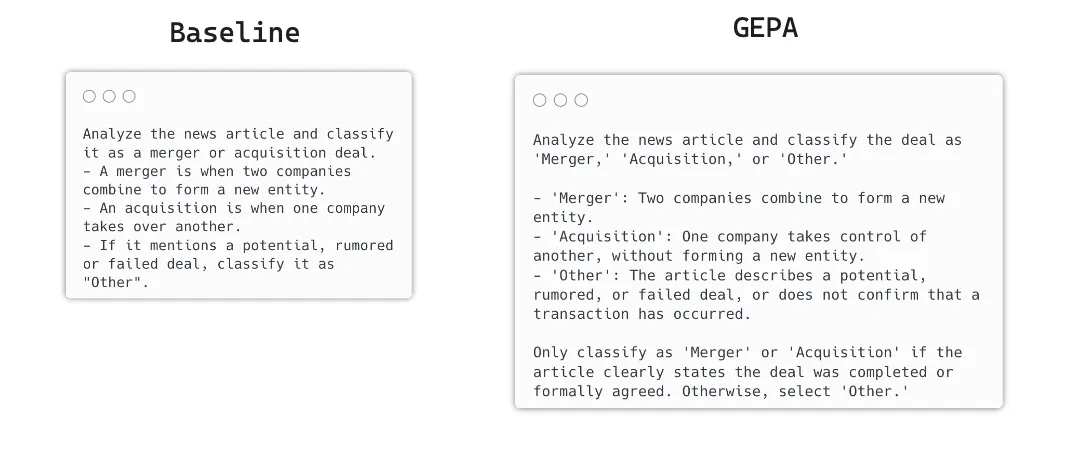
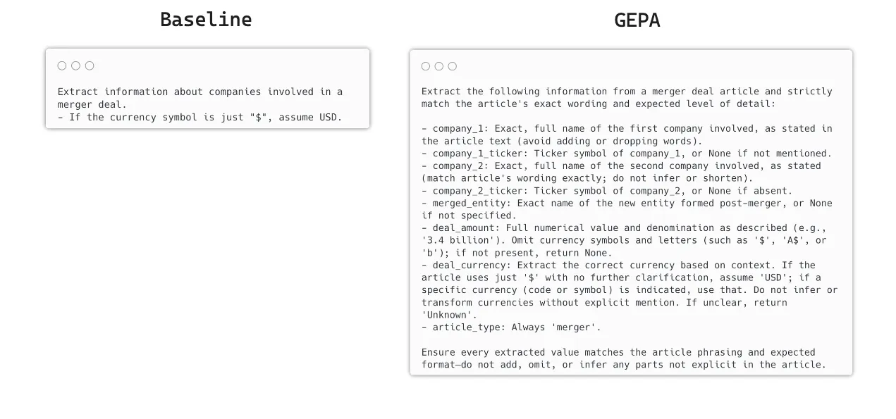
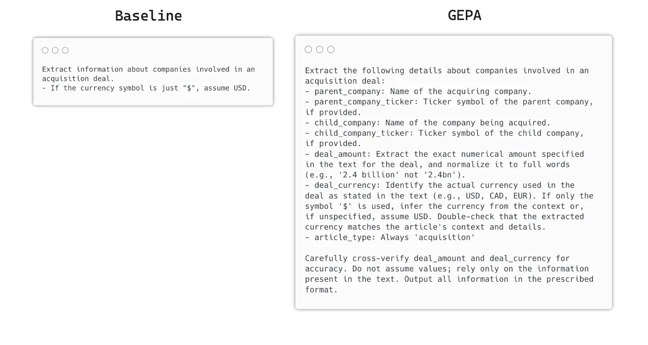
In all three tasks, GEPA was able to discover phrasing that was missing in the original human-written instructions that helped it perform the task well. For example, in the merger and acquisition information extraction tasks, GEPA discovered that it helps to explicitly mention the phrase “normalize the deal amounts to full words, e.g., 1.5 billion and not 1.5 bn”. As a human, it can be hard to know how to best phrase these kinds of instructions for the given LM. GEPA is able to use the feedback from the metric function to reason over why a previous instruction didn’t work, and is thus able to algorithmically explore a very large space of possible instructions (far larger than any human could do in reasonable time).
Cost implications#
Below, we can summarize the cost implications of the optimizer-based approach vs. human prompt engineering, which is the traditional way to improve prompts in the real world. As we all know, human time is very expensive, in comparison to machine time.
| Scenario | Rough cost | Time |
|---|---|---|
| Bootstrap fewshot optimization | <1 USD | <1 min |
| GEPA optimization | 1-10 USD | 30-90 mins |
| Human-engineered prompts | 100-1000 USD and beyond | hours to days |
The better that language models get, the more time and cost-effective it becomes to use optimizers like GEPA to automatically improve prompts, rather than relying on human ingenuity. This is especially true for complex tasks that involve structured outputs, multi-step reasoning, or tool use, where prompt engineering can be a finicky and time-consuming process.
Best practices for optimization#
These are some best practices I follow when working through a DSPy workflow. It all starts with signatures and modules!
-
Write good signatures and modules first, before worrying about optimization. The first task in DSPy is to get a working program that runs end-to-end, even if the performance is suboptimal. This is what will form the baseline result, from which we can improve.
-
Create high-quality examples that will help evaluate the system. The examples should be representative of the real-world data that the system will encounter, and should cover a good mix of edge cases and failure modes. The good news — to begin, all you need is a few dozen examples, so it’s not too onerous to hand-curate an LLM-generated synthetic dataset for almost any use case!
-
Define a good metric function that captures the essence of the task. In this case, it was an average exact match score, but for more subjective tasks, it could be an LLM-based judge that scores the output.
-
Divide the examples into uniformly distributed train and test sets (and validation sets if using GEPA). The train set is used to optimize the program, the validation set is used to evaluate candidate programs during optimization (with GEPA), and the test set is held-out (unseen during training), and used to evaluate the final optimized program. By ensuring a uniform distribution of examples across the different types of articles, we ensure that the optimizer learns from a wide variety of examples during training.
-
As more data from the real world becomes available, augment the train/validation samples with the new data, and re-run the optimizer to further improve the program. Just like in traditional machine learning, the data distribution may shift over time, or new edge cases may emerge, so we are rapidly entering the realm of continuously self-improving systems!
Using a combination of these best practices, it should be possible to get good results with DSPy optimizers right off the bat for most use cases.
Conclusions#
In this post, we looked at two optimizers in DSPy — bootstrap fewshot and GEPA — and showed how they can be used to improve the performance of an M&A information extraction pipeline from an initial baseline score of 80.7%, to 90% and then 97.8% with a light GEPA run. With heavier GEPA runs, it should be possible to get even closer to 100%.
The results are once again summarized below:
- Student model:
google/gemini-2.5-flash-lite - Teacher/Reflection model:
openai/gpt-4.1
| Case | Average Exact Match Score |
|---|---|
| Baseline | 80.7% |
| Bootstrap Fewshot | 90.7% |
| GEPA (light) | 97.8% |
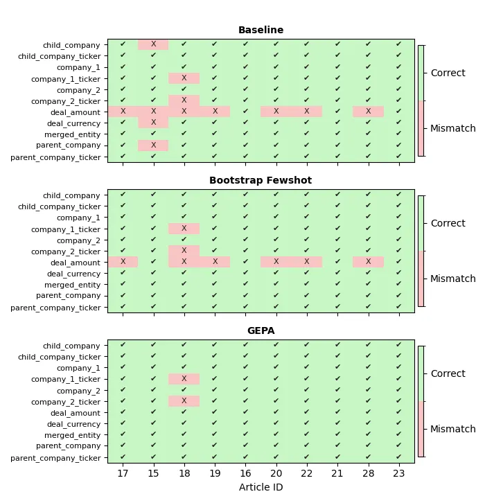
The figure below demonstrates the power of GEPA in comparison to bootstrap fewshot, and the baseline
instructions. GEPA is able to get the small google/gemini-2.5-flash-lite
model to perform well on almost all articles, with only one article’s stock tickers being incorrectly
extracted.
The future looks bright#
DSPy and its optimization ecosystem are rapidly improving, with new optimizers and techniques being added on a regular basis. From a cost and time-saving perspective, it’s becoming clearer and clearer that optimizers will play an increasingly important role in building more reliable and effective AI systems, especially as language models continue to improve in parallel.
GEPA itself continues to improve on a daily basis. This post only scratched the surface of what one can do with GEPA — stay tuned for more posts on using it for other kinds of tasks! In the future, GEPA is expected to help developers with full-program optimization (i.e., improving not just the prompts, but also the arrangement of modules), and even more performance improvements to boost rollout efficiency (so that more mutations can be generated, explored and weeded out, faster). Just like LMs are getting better, faster and cheaper over time, so too are optimizers!
Recall that part 1 of this series highlighted the great abstractions that DSPy provides, and part 2 probed into its internals. The power of a DSPy program lies in the fact that its core primitives (signatures & modules) remain unchanged over time — as new optimizers (or better versions of existing ones) come out, the performance of the program can be improved without having to change the structure of the program. The future looks bright for continuously self-improving AI systems! 🚀
Join the DSPy community online!#
My favourite part about DSPy is its awesome community online. Follow the @DSPyOSS ⤴ account on X, and join the DSPy Discord server ⤴ to learn from other really smart people! There’s never been a better time to build in the open! 😁
Code#
All code for the M&A extraction pipeline shown in this series, including optimization with bootstrap fewshot and GEPA, is available in this GitHub repo ⤴.
Footnotes#
-
One of the best parts about DSPy’s programming model and its composability is that you can jointly optimize multiple submodules (that form a larger module) using just a single set of training examples for the overall task! This is far preferable to optimizing each submodule in isolation (which would mean gathering separate datasets for each submodule), which would be impractical for most real-world tasks. ↩
-
DSPy LM calls are cached by default, to avoid incurring unnecessary costs during development and debugging. During optimization, this behaviour needs to be circumvented to ensure that the optimizer sees fresh results from each LM call. ↩