In a previous post on Lance, I described why a new columnar, multimodal lakehouse format is a compelling storage layer for AI data. In a follow-up DataFusion post, I looked at how reusable query engines let new systems target logical plans instead of rebuilding execution from scratch. In September 2025, I learned about the lance-graph ⤴ project, a Cypher-capable graph query engine built on top of Lance, which was immediately exciting because of what it represents.
At my past roles, I’ve spent a fair amount of time working with graph databases. I’ve noticed that compared to relational databases, graph databases tend to have more limited adoption across the industry, largely due to the following two facts:
- Not all query workloads benefit from a graph data model (SQL joins work just fine for most cases)
- Many teams already have a relational database or lakehouse that serves as the “source of truth,” so they want to avoid duplicating data in a separate graph database.
The modern lakehouse tends to decouple storage and compute, unlike traditional databases, where they’re tightly coupled. These days, we’re seeing a variety of standalone query engines that allow the same underlying data to support different query languages and modeling paradigms without forcing data to live in multiple systems.
lance-graph sits right at the intersection of those ideas: Lance stores the data, while DataFusion provides the planning and execution layer that graph queries can be translated into. The result is one unified storage layer that can hold multimodal data natively, support fast vector search, and, with the right graph layer and indexes on top, serve graph traversal-style queries too.
Not a separate graph database#
The easiest way to understand lance-graph as a query engine is to begin with the data itself. Nodes and edges live as Lance tables. A Person node table might have an ID column, scalar properties like name or age, embedding columns, and even multimodal assets like images. A FOLLOWS edge table might have source and target ID columns, plus its own relationship properties. Nothing about this requires a custom graph storage format.
GraphConfig is the abstraction that tells lance-graph how to interpret those tables as a property graph. It maps node labels and relationship types to tables, and identifies the columns used for node IDs, source IDs, and target IDs. The Cypher query then describes the graph pattern the user wants to match, while GraphConfig explains how that pattern maps back to ordinary columns.
At query time, lance-graph parses Cypher and validates it against this mapping. It then builds a graph-shaped plan in its own terms: start from a set of nodes, traverse one or more relationships, apply filters, and return selected properties. That intermediate step is useful because Cypher is expressed in graph vocabulary, while DataFusion expects relational operators. Once the graph pattern has been made explicit, lance-graph translates it into a DataFusion logical plan over the underlying Lance-backed tables. The flow looks roughly like this:
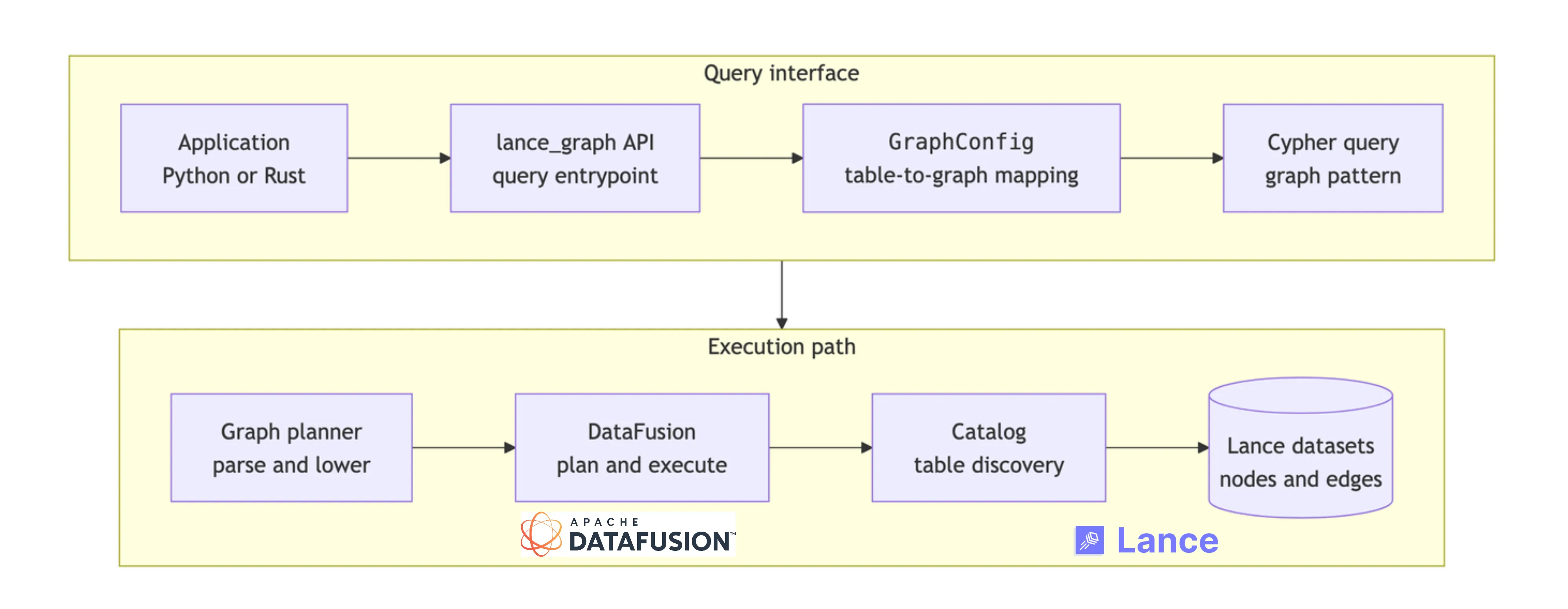
This architecture works because the responsibilities are cleanly separated. Lance stores portable, versioned, columnar datasets. DataFusion provides the reusable query execution machinery. lance-graph supplies the graph-specific frontend: the property graph mapping, Cypher parsing, semantic checks, and lowering into executable plans. For users, the payoff is that graph traversal becomes another way to compute over the same Lance-backed data, rather than a reason to create and maintain a separate graph copy.
How data mapping works#
The data mapping is easier to illustrate with a small example. As a user, you keep node and relationship data in tables, then describe how those tables should be interpreted as a graph. In the example below, Person is a node label and FOLLOWS is a relationship type. The person_id column identifies nodes, while src_person_id and dst_person_id define the direction of each edge.
import pyarrow as pa
from lance_graph import CypherQuery, GraphConfig

people = pa.table({
    "person_id": [1, 2, 3],
    "name": ["Alice", "Bob", "Carol"],
    "age": [34, 29, 41],
})

follows = pa.table({
    "src_person_id": [1, 3],
    "dst_person_id": [2, 2],
    "since": [2021, 2023],
})

config = (
    GraphConfig.builder()
    .with_node_label("Person", "person_id")
    .with_relationship("FOLLOWS", "src_person_id", "dst_person_id")
    .build()
)
The example uses in-memory Arrow tables to keep it simple, but the same shape applies when those tables are Lance datasets on disk or object storage. The important point is that columns in each table are properties on a node or relationship. There’s no need to copy them into a graph-specific JSON-like format.
Once the mapping exists, the query can be written in graph terms:
datasets = {
    "Person": people,
    "FOLLOWS": follows,
}

query = """
MATCH (a:Person)-[:FOLLOWS]->(b:Person)
WHERE a.age > 30
RETURN a.name AS follower, b.name AS followed
"""

result = CypherQuery(query).with_config(config).execute(datasets)
print(result.to_pylist())
From an ergonomics standpoint, this is a win. The data still looks like tables to Lance and DataFusion, but the application can ask relationship-shaped questions in Cypher, all without the added complexity of maintaining (and paying for) a separate graph database. GraphConfig is the bridge between those two views of the same data.
From Python calls to Rust plans#
The Python API is intentionally thin. When you write CypherQuery(...).with_config(config).execute(datasets), most of the real work happens in Rust, for obvious performance reasons. The bridge is PyO3 ⤴, which lets Rust types be exposed as Python classes while still keeping the planning and execution path inside the lance-graph ⤴ Rust crate.
At a high level, the Python CypherQuery object is a wrapper around the Rust query object:
#[pyclass(name = "CypherQuery", module = "lance.graph")]
pub struct CypherQuery {
    inner: RustCypherQuery,
}
When .execute() is called, the PyO3 layer converts the Python inputs into Arrow data structures that Rust can work with, runs the query through the Rust engine, and converts the result back into a PyArrow table. This keeps the Python surface ergonomic while leveraging Rust’s performance under the hood.
Inside Rust, the pipeline is roughly:
let semantic = SemanticAnalyzer::new(config.clone()).analyze(&ast, ¶meters)?;
let graph_plan = LogicalPlanner::new(config).plan(&semantic.ast)?;
let df_plan = DataFusionPlanner::with_catalog(config.clone(), catalog).plan(&graph_plan)?;The first step checks that the query makes sense against the declared graph model. The second turns the Cypher pattern into a graph-shaped plan. The third translates that graph plan into a DataFusion logical plan, which is where the execution machinery takes over.
Where DataFusion does the heavy lifting#
As described in the earlier post, relying on DataFusion under the hood gives system builders a reusable query engine that they don’t have to implement from scratch: it comes with built-in logical planning, optimization, physical planning, and Arrow-native execution. Once the graph layer has turned a Cypher pattern into relational work, DataFusion can take over the “hard middle” of query execution, while offering all its performance benefits.
Take the query from the previous section:
MATCH (a:Person)-[:FOLLOWS]->(b:Person)
WHERE a.age > 30
RETURN a.name AS follower, b.name AS followed
Conceptually, this becomes a join-shaped plan over three tables: the source Person table, the FOLLOWS relationship table, and the target Person table.
SELECT
  a.name AS follower,
  b.name AS followed
FROM person AS a
JOIN follows AS r ON a.person_id = r.src_person_id
JOIN person AS b ON r.dst_person_id = b.person_id
WHERE a.age > 30
Using DataFusion also means lance-graph doesn’t have to expose only one query surface. Cypher gives you graph ergonomics, while SqlQuery and SqlEngine let you work directly with SQL over the same registered tables when that’s the clearer expression:
from lance_graph import CypherQuery, SqlDialect, SqlQuery

sql = """
SELECT
  a.name AS follower,
  b.name AS followed
FROM person AS a
JOIN follows AS r ON a.person_id = r.src_person_id
JOIN person AS b ON r.dst_person_id = b.person_id
WHERE a.age > 30
"""

result = SqlQuery(sql).execute(datasets)

spark_sql = (
    CypherQuery(query)
    .with_config(config)
    .to_sql(datasets, dialect=SqlDialect.Spark)
)
Understanding performance#
How do we know if lance-graph actually performs well in practice? To study this, I ran two graph benchmark query suites: a smaller synthetic social graph in graph-benchmark ⤴, and a larger LDBC-style suite in graph-benchmark-ldbc ⤴. The results are quite interesting!
Benchmark 1: A synthetic social graph#
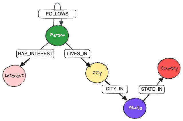
The dataset models people, interests, and locations. Person nodes follow other people, live in cities, and have interests; cities roll up into states and countries. The benchmark compares lance-graph against Neo4j Community Edition, Kuzu, and Ladybug, using a mix of leaderboard-style aggregations, filtered traversals through locations and interests, and two-hop path-counting queries.
The results are shown in the plot below. lance-graph does very well across most of the suite, especially the filtered traversal and aggregation queries where the work maps cleanly onto scans, joins, projections, and grouped aggregation. That’s exactly where the combination of DataFusion’s optimizer and Lance’s columnar storage should shine.
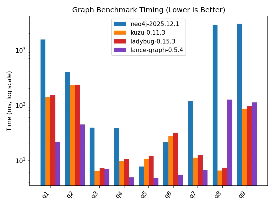
The hardest cases are Q8 and Q9, which count large numbers of two-hop paths. Q9 is especially interesting because the query shape is simple, but the intermediate path set can be huge:
MATCH (a:Person)-[r1:FOLLOWS]->(b:Person)-[r2:FOLLOWS]->(c:Person)
WHERE b.age < $age_1 AND c.age > $age_2
RETURN count(*) AS numPaths
This is exactly the kind of query that Kuzu (and its fork Ladybug) excel at, because it benefits from factorized joins1. A straightforward execution strategy has to consider matching (a, b, c) triples, while a factorized strategy can reason more compactly in terms of filtered in-degrees and out-degrees around the middle node b. Kuzu’s execution engine is designed around a hybrid of worst-case optimal joins, binary joins, and factorization. What’s remarkable, however, is that lance-graph performs respectably well on Q8/Q9 despite not being a specialized graph engine built from scratch.
Benchmark 2: LDBC SNB SF1#
The second benchmark, graph-benchmark-ldbc ⤴, uses the LDBC Social Network Benchmark dataset at scale factor 1. This is a more realistic stress test than the synthetic social graph: the dataset has roughly 3.1 million nodes, 17 million relationships, 8 node types, and 23 relationship types. The query suite contains 30 Cypher queries with a wider range of traversal lengths, relationship types, cardinalities, filters, and projections.
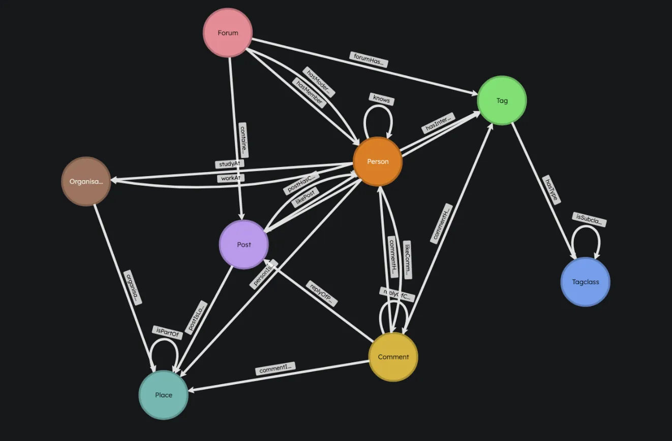
The value of this benchmark is that it exercises more of the graph query surface. Instead of only asking about Person-to-Person follower paths, the queries touch posts, comments, forums, tags, places, organizations, memberships, likes, replies, and creator/location relationships. This creates a much broader mix of join shapes and selectivity patterns.
| Query | neo4j-2025.12.1 (ms) | kuzu-0.11.3 (ms) | ladybug-0.15.3 (ms) | lance-graph-0.5.4 (ms) |
|---|---|---|---|---|
| q1 | 4.9ms | 2.3ms (2.2x) | 3.4ms (1.4x) | 2.3ms (2.1x) |
| q2 | 5.9ms | 1.4ms (4.1x) | 2.3ms (2.6x) | 3.3ms (1.8x) |
| q3 | 2.9ms | 1.2ms (2.4x) | 2.0ms (1.5x) | 3.1ms (0.9x) |
| q4 | 4.1ms | 1.0ms (4.0x) | 1.6ms (2.5x) | 4.2ms (1.0x) |
| q5 | 4.9ms | 3.8ms (1.3x) | 5.9ms (0.8x) | 3.0ms (1.6x) |
| q6 | 3.9ms | 0.8ms (5.0x) | 1.4ms (2.8x) | 1.3ms (2.9x) |
| q7 | 2.2ms | 31.1ms (0.1x) | 50.1ms (0.0x) | 19.1ms (0.1x) |
| q8 | 14.6ms | 2.9ms (5.1x) | 4.5ms (3.2x) | 2.0ms (7.4x) |
| q9 | 2.8ms | 2.1ms (1.4x) | 3.5ms (0.8x) | 3.4ms (0.8x) |
| q10 | 4.9ms | 1.8ms (2.7x) | 3.1ms (1.6x) | 32.3ms (0.2x) |
| q11 | 14.9ms | 8.5ms (1.8x) | 13.6ms (1.1x) | 5.1ms (2.9x) |
| q12 | 8.1ms | 20.7ms (0.4x) | 23.9ms (0.3x) | 22.2ms (0.4x) |
| q13 | 9.9ms | 50.8ms (0.2x) | 82.8ms (0.1x) | 11.5ms (0.9x) |
| q14 | 1.7ms | 1.7ms (1.0x) | 2.8ms (0.6x) | 4.0ms (0.4x) |
| q15 | 3.3ms | 2.7ms (1.2x) | 4.4ms (0.7x) | 3.5ms (0.9x) |
| q16 | 2.4ms | 2.0ms (1.2x) | 3.2ms (0.7x) | 5.7ms (0.4x) |
| q17 | 4.9ms | 3.0ms (1.6x) | 4.8ms (1.0x) | 3.8ms (1.3x) |
| q18 | 3.7ms | 1.8ms (2.0x) | 2.8ms (1.3x) | 3.0ms (1.2x) |
| q19 | 7.8ms | 12.4ms (0.6x) | 22.5ms (0.3x) | 25.8ms (0.3x) |
| q20 | 475.7ms | 11.9ms (39.9x) | 17.0ms (28.0x) | 3.6ms (133.5x) |
| q21 | 1.8ms | 0.6ms (3.2x) | 0.9ms (2.1x) | 2.6ms (0.7x) |
| q22 | 3.6ms | 24.2ms (0.2x) | 26.6ms (0.1x) | 16.7ms (0.2x) |
| q23 | 3.9ms | 1.4ms (2.8x) | 2.3ms (1.7x) | 3.9ms (1.0x) |
| q24 | 1.6ms | 1.5ms (1.1x) | 2.4ms (0.7x) | 2.9ms (0.6x) |
| q25 | 3.1ms | 1.8ms (1.7x) | 2.9ms (1.1x) | 2.4ms (1.3x) |
| q26 | 1.8ms | 3.7ms (0.5x) | 5.9ms (0.3x) | 4.5ms (0.4x) |
| q27 | 3.5ms | 15.2ms (0.2x) | 24.0ms (0.1x) | 32.3ms (0.1x) |
| q28 | 3.9ms | 1.7ms (2.3x) | 3.5ms (1.1x) | 4.2ms (0.9x) |
| q29 | 2.9ms | 1.3ms (2.3x) | 2.3ms (1.2x) | 3.7ms (0.8x) |
| q30 | 1255.2ms | 158.7ms (7.9x) | 231.9ms (5.4x) | 38.8ms (32.3x) |
The results are again mixed in a useful way. lance-graph is competitive across much of the suite, and it’s particularly strong on some of the larger outlier queries: q20 and q30 are the most obvious examples. But it’s not uniformly the fastest or slowest system. Some queries still favor Kuzu/Ladybug, and a few favor Neo4j, which suggests there’s plenty of room in lance-graph for future improvements in performance across a wider range of query shapes, potentially with custom optimizers.
The takeaway is the same as before, just with more confidence: lance-graph is already serious enough to compare against dedicated graph systems on a standard benchmark workload, while keeping the architecture much more composable. It’s not claiming to be the fastest graph query processor. It’s showing that a Cypher frontend, DataFusion execution, and Lance storage can form a credible graph engine without requiring users to pay for and maintain a separate graph database stack.
Towards multimodal knowledge graphs (MMKG)#
Building the graph layer on top of Lance also expands what a graph can represent. Traditional graph databases are good at entities and relationships, but modern AI applications also lean on images, video, audio, and embeddings. With Lance underneath, those payloads ride on the same node tables the graph layer queries: they’re just additional columns in Lance tables.
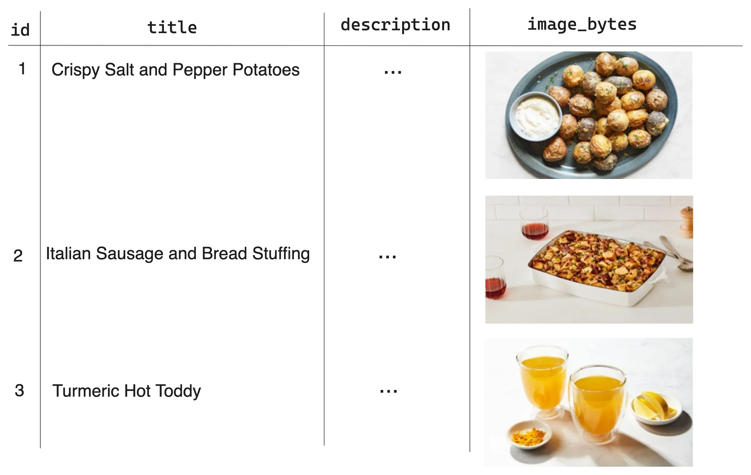
Consider a multimodal knowledge graph of recipes. The Recipe node table in Lance format carries structured fields like title and description alongside an image column of raw JPEG bytes and an image_embedding column (a 512-dim CLIP vector). The multimodal payload sits directly on the entity it belongs to.
MATCH (r:Recipe)-[:USES_INGREDIENT]->(i:Ingredient)
WHERE i.name CONTAINS 'chicken'
RETURN r.title, r.image_bytes
LIMIT 10
Cypher handles the graph-shaped work: traversing relationships, filtering on structured properties, and projecting the requested columns. Because the underlying tables are Arrow, RETURN can hand back binary blobs and vectors directly. r.image_bytes comes through as a Python bytes object (raw JPEG, ready to render), and r.image_embedding as a list of floats. There’s no second hop to an object store; the bytes already live in the same Lance table the graph just queried, riding back through the result set with the rest of the projection.
For vector search, lance-graph treats it as a complementary step rather than another Cypher clause. The typical pattern is two-stage: use Cypher to traverse the graph and narrow down to a candidate set, then rank that set with a separate VectorSearch call against an embedding column backed by a Lance ANN index. The VISUALLY_SIMILAR edges in the example above were themselves built this way at ingest time, by running top-k cosine search over image_embedding.
The convenience method that ties the two stages together is execute_with_vector_rerank. The query below uses Cypher to find recipes that use chicken, then ranks those candidates by visual similarity to a seed embedding (in this case, the embedding of the Miso-Butter Roast Chicken recipe):
from lance_graph import CypherQuery, DistanceMetric, GraphConfig, VectorSearch

cypher = """
MATCH (r:Recipe)-[:USES_INGREDIENT]->(i:Ingredient)
WHERE i.name CONTAINS 'chicken'
RETURN DISTINCT r.id, r.title, r.image_embedding
"""

results = (
    CypherQuery(cypher)
    .with_config(config)
    .execute_with_vector_rerank(
        datasets,
        VectorSearch("r.image_embedding")
        .query_vector(seed_embedding)
        .metric(DistanceMetric.Cosine)
        .top_k(5)
        .include_distance(True),
    )
)
Running this against the recipes MMKG returns the seed itself first (cosine distance 0.0), followed by other chicken recipes ranked by visual similarity:
0.0000  Miso-Butter Roast Chicken With Acorn Squash Panzanella
0.1153  Thai Muslim-Style Grilled Chicken
0.1273  Braised Chicken Legs With Grapes and Fennel
0.1598  Caesar Salad Roast Chicken
0.1702  Maple Barbecue Grilled Chicken
This showcases the “graph + vector” hybrid in one call within an MMKG: Cypher narrows the search set by ingredient relationship, and VectorSearch ranks the results by image similarity, all over the same Lance tables.
What this makes clear is that a multimodal knowledge graph feels like just another query layer over the same AI-native tables. The graph structure and the multimodal payloads live side by side in Lance, Cypher handles traversal and structured filters, and vector search plugs in alongside when you need it. No separate object store for images, no separate vector database for embeddings, and no graph-only system holding pointers to both.
Conclusions#
The deeper story here isn’t really about graphs. It’s about a quiet shift in how modern data systems are getting built. For a long time, databases were sold (and engineered) as vertically integrated stacks, with storage, indexing, planning, execution, and the query language all welded together into one system. If you wanted any of those pieces, you took the whole thing.
That model is unwinding. Apache Arrow standardized how columnar data moves around in memory, so different tools can hand each other data without serializing through an intermediate format. Lance has stepped in as a modern, AI-native table substrate that sits well on object storage and handles versioning, vector indexes, and large multimodal columns. DataFusion provides a reusable query execution engine that anyone building a new system can plug into rather than reinventing from scratch. Each of these layers is open, embeddable, and replaceable in a way the old monoliths weren’t.
lance-graph is what happens when we put those layers together and ask: do we still need a separate graph database? Or are we moving toward “graph lakehouses”? Similar ideas are showing up in other paradigms too: search, time series, and SQL itself. Query engines are increasingly becoming something we bring to our data, rather than the other way around.
As we move toward more “deconstructed data systems,” where the components of a database are available as composable building blocks, lance-graph is one concrete example of where that’s heading, and it probably won’t be the last. If you’re interested in shaping the future of multimodal knowledge graphs, lance-graph ⤴ is a good project to watch and get involved with!
Footnotes#
-
Factorized joins avoid materializing every row of a large intermediate join result when the query can be represented more compactly. In the Q9 example, instead of enumerating every
(a, b, c)path, the engine can group work around the middle nodeband combine the relevant incoming and outgoing edge counts after applying the filters. This is especially effective for path-counting queries where the number of matching paths can be much larger than the number of edges. ↩